Single-Stage Solvex Development Cortix Tech 30Sep2025
1. Use-Case 03: TBP-Diluent-H\(_2\)O-HNO\(_3\)-Air Mixing#

Developer: Valmor F. de Almeida, PhD
Cortix Tech, Lowell, MA 01854, USA
Revision date: 19Nov25
1.1. Objectives#
Develop usecase scenario for water and nitric acid extraction by TBP with a vapor phase.
Test implementation and present results.
Use AI assistants to help with information and reporting.
AI requests below may need to be executed multiple times if the result is not satisfactory or incorrect.
'''AI assistance options'''
# Set all to False if you do not have access to OpenAI API and/or AI codes below
cortix_ai = True
stage_ai = True
'''Generate proprietary knowledge database?'''
db_save = False # set this to false if going public (online) with this notebook
'''Other helpers'''
fig_count = 0
tbl_count = 0
markdown_display = True # if False code cell output is type: stream, else: markdown. Use True for in-house conversion to .md
1.2. System#
Single stage mixing of TBP with inert diluent, HNO3 solution, and vapor.
'''Setup the base system'''
from cortix import Cortix
from cortix import Network
from cortix import Units as unit
from cortix import ReactionMechanism
from cortix import Quantity

system = Cortix(use_mpi=False, splash=True) # System top level
system_net = system.network = Network() # Network

if cortix_ai:
    from cortix import CortixAI
    cortix_ai = CortixAI(llm_model='gpt-5-mini', llm_cleverness=0.8)
    cortix_ai.markdown_header_level = '<h3>'
    cortix_ai.n_chunks = 8

if cortix_ai:
    cortix_ai.explain(markdown_display=markdown_display, save_supporting_info=db_save, save_supporting_info=db_save)
[11440] 2025-11-19 23:15:26,310 - cortix - INFO - Created Cortix object
_____________________________________________________________________________
                             L A U N C H I N G
_____________________________________________________________________________
      ...                                        s       .     (TAAG Fraktur)
   xH88"`~ .x8X                                 :8      @88>
 :8888   .f"8888Hf        u.      .u    .      .88      %8P      uL   ..
:8888>  X8L  ^""`   ...ue888b   .d88B :@8c    :888ooo    .     .@88b  @88R
X8888  X888h        888R Y888r ="8888f8888r -*8888888  .@88u  ""Y888k/"*P
88888  !88888.      888R I888>   4888>"88"    8888    888E`    Y888L
88888   %88888      888R I888>   4888> "      8888      888E      8888
88888 `> `8888>     888R I888>   4888>        8888      888E      `888N
`8888L %  ?888   ! u8888cJ888   .d888L .+    .8888Lu=   888E   .u./"888&
 `8888  `-*""   /   "*888*P"    ^"8888*"     ^%888*     888&  d888" Y888*"
   "888.      :"      "Y"          "Y"         "Y"      R888" ` "Y   Y"
     `""***~"`                                           ""
                             https://cortix.org
_____________________________________________________________________________
Cortix AI assistant: working on explanation...
Overview
This snippet configures a Cortix “system” object, creates a network, and conditionally constructs and configures a CortixAI object before invoking a method on it.
Imports
The code brings symbols from the cortix package into the local namespace:
Cortix: the top-level object representing a Cortix runtime.
Network: an object representing a chemical/kinetic network.
Units as unit: the Units helper is aliased to unit.
ReactionMechanism: imported (not used in the shown snippet) for defining reaction sets.
Quantity: imported (not used in the shown snippet) for numeric/physical quantities with units.
System and network setup
system = Cortix(use_mpi=False, splash=True) creates a Cortix instance named system with two keyword arguments:
use_mpi=False disables MPI-based parallelism for this runtime.
splash=True requests the Cortix startup/banner behavior (a “splash”) during initialization.
system_net = system.network = Network() constructs a Network instance and assigns it two ways:
system.network is set to that Network instance (attaching the network to the Cortix system).
system_net is a local variable referencing the same Network object (so system_net and system.network reference identical objects).
Conditional creation and configuration of CortixAI
The code uses two guarded blocks that run only if the name cortix_ai evaluates as truthy in the current scope:
First guarded block:
from cortix import CortixAI imports the CortixAI helper/class from the cortix package.
cortix_ai = CortixAI(llm_model=’gpt-5-mini’, llm_cleverness=0.8) replaces the existing cortix_ai name with a CortixAI instance constructed with:
llm_model=’gpt-5-mini’ (selects the language model identifier supplied to CortixAI).
llm_cleverness=0.8 (a numeric configuration parameter passed to the CortixAI constructor).
cortix_ai.markdown_header_level = ‘
’ sets an attribute on the CortixAI instance to the string ‘
’.
cortix_ai.n_chunks = 8 sets another attribute on the instance to the integer 8.
Second guarded block:
cortix_ai.explain(markdown_display=markdown_display, save_supporting_info=db_save) invokes the explain method on the cortix_ai object with two keyword arguments:
markdown_display with the value of the variable markdown_display from the surrounding scope.
save_supporting_info with the value of the variable db_save from the surrounding scope.
Important runtime implications
The two if cortix_ai: checks require that the name cortix_ai is already defined and truthy before entering the first block; if cortix_ai is undefined at runtime, a NameError will be raised when evaluating the condition.
Within the first conditional, the code reassigns the name cortix_ai to a CortixAI instance, shadowing whatever earlier value cortix_ai had.
The snippet references markdown_display and db_save when calling cortix_ai.explain; those names must exist in the surrounding scope to avoid NameError at call time.
ReactionMechanism and Quantity are imported but not used in the visible fragment; they are available for later use in the same module.
AI Parameters:
+ LLM model (OpenAI) = gpt-5-mini
+ LLM cleverness     = 1.0
+ Total # of tokens  = 3678
'''FYI LLM models info'''
if cortix_ai:
    print(cortix_ai.llm_names_info)
{'gpt-5': 'Full reasoning-intensive tasks', 'gpt-5-mini': 'Balance of speed and capability', 'gpt-5-nano': 'Speed and cost efficiency', 'gpt-4o-mini': 'Fastest at advanced reasoning', 'gpt-4o': 'Great for most tasks', 'gpt-4.1': 'Great for quick coding and analysis', 'gpt-4.1-mini': 'Faster than 4.1 for everyday tasks'}
1.2.1. Stage#
Instantiate a single stage to model and simulate the reactive mixing process.
'''Import Stage'''
from solvex import Stage
'''Create and configure a StageAI object'''
if stage_ai:
    from stage_ai import StageAI
    stage_ai = StageAI(llm_model='gpt-5-mini', llm_cleverness=0.8)
    stage_ai.markdown_header_level = '<h4>'
if stage_ai:
    stage_ai.help('stage', markdown_display=markdown_display, save_supporting_info=db_save)
Stage AI assistant: working on help...
Stage Description
Module overview
This Stage module models a single solvent-extraction contactor with three interacting phases (aqueous, organic, vapor). It integrates a time-dependent mass-balance system using scipy.integrate.odeint and organizes state/history in phase containers. The module supports connecting ports to other modules and exchanging mass-rate information during time stepping.
Phases involved
aqueous phase
organic phase
vapor phase
Information about a stage module is needed: stage
Original Stage schematics
                          Aqueous    Organic
                         External    Product
                           Feed
                             |          ^
                             |          |
                             |          |
                             V          |
                        |---------------------|
   Vapor/Org inter-stage|                     | Vapor/Aqu inter-stage
   outflow <------------|                     |-----------> outflow
                        |                     |
   Organic inter-stage  |    S O L V E N T    | Aqueous inter-stage
   outflow <------------| E X T R A C T I O N |-----------> outflow
                        |                     |
                        |                     |
   Vapor/Aqu inter-stage|      S T A G E      | Vapor/Org inter-stage
   inflow  ------------>|                     |<----------- inflow
                        |                     |
   Aqueous inter-stage  |                     | Organic inter-stage
   inflow ------------->|                     |<----------- inflow
                        |---------------------|
                             |          ^
                             |          |
                             |          |
                             V          |
                          Aqueous    Organic
                          Product    External
                                       Feed
Source structure and primary components
Module class: Stage (inherits cortix.Module)
Phases: stored as Phase containers; there are both state phases and inflow-parameter phases
Reaction mechanism: optional ReactionMechanism attached via add_reaction_mechanism
Time integration: run() orchestrates stepping; internal __step() advances the ODE system
Mass-balance RHS: provided by __mbal_rhs_func (used by odeint)
Port interactions: ports exist and are invoked in __call_ports() before/after stepping
Ports (existence)
Ports are defined (expected) by the module and used to exchange mass-rate vectors. Example (one-line python list of expected port names):
[‘aqu-feed’, ‘org-feed’, ‘aqu-product’, ‘org-product’, ‘aqu-inflow’, ‘org-inflow’, ‘aqu-outflow’, ‘org-outflow’, ‘vap-aqu-inflow’, ‘vap-org-inflow’, ‘vap-aqu-outflow’, ‘vap-org-outflow’]
Notes regarding ports and communication:
The run loop calls __call_ports(time) each step to send/recv messages from connected ports.
Typical patterns: recv() an inflow mass-rate vector from an inflow port; send() an outflow request or data to outflow/product ports.
The module checks port.connected_port to decide whether to perform communication.
Key classes & method signatures (not full source)
class Stage(Module)
init(self, mix_vol, vol_flowrates, temperature)
add_reaction_mechanism(self, rxn_mech=None)
run(self, *args)
__call_ports(self, time)
__step(self, time=0.0)
__get_state_vector(self, time=None, cc_name=’mass_cc’)
__mbal_rhs_func(self, u_vec, time, params)
__update_outflow_mass_rates(self, u_vec)
__convert_mass_cc_to_molar_cc(self, u_vec)
__update_state_variables(self, u_vec, time)
r_vec(self, time=None)
g_vec(self, time=None)
rxn_efficiencies(self, time=None)
(many private helpers and Phase setup methods)
The step method: purpose and snippet
Purpose:
Assembles the current state vector, calls the ODE integrator over the next time interval, checks integration success and mass conservation, optionally computes mass-flowrate diagnostics, and updates the phase containers with the new state.
Step method snippet (illustrative excerpt):
def __step(self, time=0.0):
    """Stepping Stage in time."""
    u_vec_0 = self.__get_state_vector(time)
    t_interval = np.linspace(time, time+self.time_step, num=2)

    (u_vec_hist, info_dict) = odeint(self.__mbal_rhs_func,
                                     u_vec_0, t_interval,
                                     args=(self.__ode_params,),
                                     full_output=True )

    assert info_dict['message'] == 'Integration successful.'
    u_vec = u_vec_hist[1,:]

    time += self.time_step

    # mass conservation checks (optional)
    self.__check_mass_conservation(u_vec, write=(self.monitor_mass_conservation_residual or time >= self.end_time))

    # update history containers
    self.__update_state_variables(u_vec, time)

    return time
(higher-level details omitted; this snippet shows the integration and update flow)
Mass-balance RHS function: role and signature
Signature: __mbal_rhs_func(self, u_vec, time, params)
Role:
This function computes the right-hand side dt_u of the ODE system used by odeint.
Responsibilities inside the function include:
Enforce non-negativity of u_vec entries (u_vec[u_vec < 0.0] = 0.0).
Update outflow mass rates derived from the current u_vec via __update_outflow_mass_rates(u_vec).
Convert mass concentrations to molar concentrations for reaction calculations (__convert_mass_cc_to_molar_cc).
Call the reaction mechanism (self.rxn_mech.g_vec(…)) to obtain species generation rate densities g_vec.
For each phase (aqueous, organic, vapor) compute dt for all species combining inflow, outflow and generation terms. Typical formula per species: dt_u[gidx] = ((mass_inflow_rate - mass_outflow_rate)/mixing_vol + g_vec[gidx] * M) / phi where phi is the phase volume fraction and M is species molar mass.
Return the assembled dt_u numpy array to the integrator.
Ports, communication and time stepping interaction
run() orchestrates the simulation time loop. Within each loop iteration:
Optionally perturb inflow rates (randomization) via __perturb_mass_inflow_rates().
Call __step(time) to integrate for one time_step.
Call __call_ports(time) to exchange information with connected modules (send/recv).
__call_ports handles the port-level protocol: it checks for a connected_port, performs send(time,’port_name’) to request or provide data, and recv(‘port_name’) to obtain mass-rate arrays. Received vectors are validated for expected length before being used.
Inflows are kept as parameter-phase containers (inflow_aqueous_phase, inflow_organic_phase, inflow_vapor_), and their concentrations are used to compute species_inflow_mass_rates_ before stepping.
Typical usage snippet
# create a Stage with mixing volume, volumetric flowrates and temperature (SI units from Units)
stg = Stage(mix_vol, vol_flowrates, temperature)
# add reaction mechanism
stg.add_reaction_mechanism(rxn_mech)
# connect ports externally or leave inflow parameters set locally
# run the transient simulation: run expects an args tuple with at least logger info in this implementation
stg.run((some_logger,))
(higher-level connection API: use Module.get_port/send/recv to wire stages together)
Data access and diagnostics
State/history is stored per phase (phase.add_row). Methods return Quantity objects for histories: mass_density_history(), r_vec_history(), g_vec_history(), efficiency_history().
The module offers monitoring toggles: monitor_mass_flowrates and monitor_mass_conservation_residual that print or assert diagnostics at runtime.
Summary
The Stage module implements a time-integrated, phase-resolved mass-balance model for solvent extraction with aqueous, organic and vapor phases.
Time evolution is done by assembling a global state vector, invoking odeint with __mbal_rhs_func, validating mass conservation and updating Phase history containers.
Ports exist to connect inflows/outflows to other modules; the run loop invokes __call_ports to exchange mass-rate vectors during stepping.
Key interfaces to inspect or visualize results include r_vec(), g_vec(), rxn_efficiencies() and various “_history” methods.
AI Parameters:
+ LLM model (OpenAI) = gpt-5-mini
+ LLM cleverness     = 1.0
+ RAG                = stage.py
+ Total # of tokens  = 17612
Done with help...
1.2.1.1. Configuration#
'''Create Stage and add to base system'''

# Initialization
mixing_volume = 1*unit.L
# Aqueous phase
vol_flowrate_aqu = 500*unit.mL/unit.min
# Organic phase
vol_flowrate_org = 600*unit.mL/unit.min
# Vapor phase
vol_flowrate_vap = (3.7*vol_flowrate_org/100, 8.1*vol_flowrate_aqu/100) # percentage of (org, aqu)

vol_flowrates = [vol_flowrate_org, vol_flowrate_aqu, vol_flowrate_vap]

stg_temperature = unit.convert_temperature(40, 'C', 'K')

stg = Stage(mixing_volume, vol_flowrates, stg_temperature) # Create solvent extraction module

system_net.module(stg) # Add stage module to network

if cortix_ai:
    cortix_ai.explain(markdown_header_level='<h5>', markdown_display=markdown_display, save_supporting_info=db_save)
Cortix AI assistant: working on explanation...
Overview
The script builds a solvent-extraction “Stage” instance with specified mixing volume, phase volumetric flowrates, and temperature, then registers that stage with a system network and conditionally calls a method on a cortix_ai object.
Top-level constants and units
A module-level docstring/comment indicates intent: “Create Stage and add to base system”.
mixing_volume is set to 1 L (1*unit.L), representing the stage mixing volume as a quantity with units.
vol_flowrate_aqu is set to 500 mL/min (500*unit.mL/unit.min) for the aqueous phase, and vol_flowrate_org is set to 600 mL/min for the organic phase.
vol_flowrate_vap is a tuple of two computed quantities: (3.7% of the organic flow, 8.1% of the aqueous flow); each element is computed by multiplying the percentage by the corresponding flow and dividing by 100.
vol_flowrates is a list combining the three phase flows in order: [organic, aqueous, vapor].
stg_temperature is obtained by converting 40 °C to kelvin via unit.convert_temperature(40, ‘C’, ‘K’), yielding a temperature quantity in K.
Object creation and registration
stg = Stage(mixing_volume, vol_flowrates, stg_temperature) constructs a Stage object (presumably a solvent-extraction module) with the mixing volume, the list of volumetric flowrates, and the stage temperature as arguments.
system_net.module(stg) attaches or registers the created Stage instance with the system network object named system_net.
Control flow and conditional call
The final if-block checks the truthiness of cortix_ai; if true, it calls a method on that object with three keyword arguments (markdown_header_level set to ‘
’, markdown_display passed through, and save_supporting_info provided as db_save).
AI Parameters:
+ LLM model (OpenAI) = gpt-5-mini
+ LLM cleverness     = 1.0
+ Total # of tokens  = 3227
print('Flow residence time [s]: average = %5.3e'%stg.flow_residence_time_avg)
print('Aqueous volume fraction = %5.3e'%stg.volume_frac_aqu)
print('Organic volume fraction = %5.3e'%stg.volume_frac_org)
print('Vapor volume fraction   = %5.3e'%stg.volume_frac_vap)
Flow residence time [s]: average = 5.160e+01
Aqueous volume fraction = 4.300e-01
Organic volume fraction = 5.160e-01
Vapor volume fraction   = 5.393e-02
'''Draw the Cortix network system'''
system_net.draw(engine='circo', node_shape='folder', ports=True)

'''For help purposes'''
import solvex.stage
Documentation options:
Live in this notebook run on code cell:
help(solvex_ustc.stage)On the web: source
# Poor's man help
#help(solvex_ustc.stage)
1.2.2. Reaction Mechanism#
Contacting water, inert diluent and TBP, nitric acid, and air.
1.2.2.1. Nitric acid, water extraction example#
args_dict = {'water_activity': 1.0}
file_name = 'tbp-h2o-hno3-air.txt'
rxn_mech = ReactionMechanism(file_name=file_name, order_species=True, args_dict=args_dict)
WARNING: ReactionMechanism: user must implement a H2O*[C4H9O]3PO(o) product partition function with signature <product>(rxn_mech, temperature, spc_molar_cc, arg_dict) function for [C4H9O]3PO(o) + H2O(a) <-> H2O*[C4H9O]3PO(o)
WARNING: ReactionMechanism: user must implement a [H2O]2*[[C4H9O]3PO]2(o) product partition function with signature <product>(rxn_mech, temperature, spc_molar_cc, arg_dict) function for 2 [C4H9O]3PO(o) + 2 H2O(a) <-> [H2O]2*[[C4H9O]3PO]2(o)
WARNING: ReactionMechanism: user must implement a [H2O]6*[[C4H9O]3PO]3(o) product partition function with signature <product>(rxn_mech, temperature, spc_molar_cc, arg_dict) function for 3 [C4H9O]3PO(o) + 6 H2O(a) <-> [H2O]6*[[C4H9O]3PO]3(o)
WARNING: ReactionMechanism: user must implement a HNO3*[C4H9O]3PO(o) product partition function with signature <product>(rxn_mech, temperature, spc_molar_cc, arg_dict) function for H^+(a) + NO3^-(a) + [C4H9O]3PO(o) <-> HNO3*[C4H9O]3PO(o)
WARNING: ReactionMechanism: user must implement a HNO3*[[C4H9O]3PO]2(o) product partition function with signature <product>(rxn_mech, temperature, spc_molar_cc, arg_dict) function for H^+(a) + NO3^-(a) + 2 [C4H9O]3PO(o) <-> HNO3*[[C4H9O]3PO]2(o)
WARNING: ReactionMechanism: user must implement a H2O(v) product partition function with signature <product>(rxn_mech, temperature, spc_molar_cc, arg_dict) function for H2O(a) <-> H2O(v)
WARNING: ReactionMechanism: user must implement a O2(a) product partition function with signature <product>(rxn_mech, temperature, spc_molar_cc, arg_dict) function for O2(v) <-> O2(a)
WARNING: ReactionMechanism: user must implement a N2(a) product partition function with signature <product>(rxn_mech, temperature, spc_molar_cc, arg_dict) function for N2(v) <-> N2(a)
#'''User input'''
#rxn_mech.cat_input()
#'''Show Mechanism'''
# Jupyter Book does not render LaTeX through IPython.display(Markdown)
rxn_mech.md_print()
14 Species:
\begin{align*}
&{\mathrm{H}{2}\mathrm{O}}\mathrm{(a)} \quad {\mathrm{H}{2}\mathrm{O}}\mathrm{(v)} \quad {\mathrm{H}{2}\mathrm{O}\bullet[\mathrm{C}{4}\mathrm{H}{9}\mathrm{O}]{3}\mathrm{P}\mathrm{O}}\mathrm{(o)} \quad {\mathrm{H}\mathrm{N}\mathrm{O}{3}\bullet[\mathrm{C}{4}\mathrm{H}{9}\mathrm{O}]{3}\mathrm{P}\mathrm{O}}\mathrm{(o)} \quad {\mathrm{H}\mathrm{N}\mathrm{O}{3}\bullet[[\mathrm{C}{4}\mathrm{H}{9}\mathrm{O}]{3}\mathrm{P}\mathrm{O}]{2}}{\mathrm{(o)}} \quad {\mathrm{H}^+}\mathrm{(a)} \quad {\mathrm{N}{2}}{\mathrm{(a)}} \quad {\mathrm{N}{2}}{\mathrm{(v)}} \quad \
& {\mathrm{N}\mathrm{O}{3}^-}\mathrm{(a)} \quad {\mathrm{O}{2}}{\mathrm{(a)}} \quad {\mathrm{O}{2}}{\mathrm{(v)}} \quad {[\mathrm{C}{4}\mathrm{H}{9}\mathrm{O}]{3}\mathrm{P}\mathrm{O}}\mathrm{(o)} \quad {[\mathrm{H}{2}\mathrm{O}]{2}\bullet[[\mathrm{C}{4}\mathrm{H}{9}\mathrm{O}]{3}\mathrm{P}\mathrm{O}]{2}}{\mathrm{(o)}} \quad {[\mathrm{H}{2}\mathrm{O}]{6}\bullet[[\mathrm{C}{4}\mathrm{H}{9}\mathrm{O}]{3}\mathrm{P}\mathrm{O}]{3}}_{\mathrm{(o)}}\end{align*}
8 Reactions: \begin{align*} {\mathrm{H}{2}\mathrm{O}}\mathrm{(a)}\ + \ {[\mathrm{C}{4}\mathrm{H}{9}\mathrm{O}]{3}\mathrm{P}\mathrm{O}}\mathrm{(o)}\ &\longleftrightarrow \ {\mathrm{H}{2}\mathrm{O}\bullet[\mathrm{C}{4}\mathrm{H}{9}\mathrm{O}]{3}\mathrm{P}\mathrm{O}}\mathrm{(o)}\ 2.0,{\mathrm{H}{2}\mathrm{O}}\mathrm{(a)}\ + \ 2.0,{[\mathrm{C}{4}\mathrm{H}{9}\mathrm{O}]{3}\mathrm{P}\mathrm{O}}\mathrm{(o)}\ &\longleftrightarrow \ {[\mathrm{H}{2}\mathrm{O}]{2}\bullet[[\mathrm{C}{4}\mathrm{H}{9}\mathrm{O}]{3}\mathrm{P}\mathrm{O}]{2}}{\mathrm{(o)}}\ 6.0,{\mathrm{H}{2}\mathrm{O}}\mathrm{(a)}\ + \ 3.0,{[\mathrm{C}{4}\mathrm{H}{9}\mathrm{O}]{3}\mathrm{P}\mathrm{O}}\mathrm{(o)}\ &\longleftrightarrow \ {[\mathrm{H}{2}\mathrm{O}]{6}\bullet[[\mathrm{C}{4}\mathrm{H}{9}\mathrm{O}]{3}\mathrm{P}\mathrm{O}]{3}}{\mathrm{(o)}}\ {\mathrm{H}^+}\mathrm{(a)}\ + \ {\mathrm{N}\mathrm{O}{3}^-}\mathrm{(a)}\ + \ {[\mathrm{C}{4}\mathrm{H}{9}\mathrm{O}]{3}\mathrm{P}\mathrm{O}}\mathrm{(o)}\ &\longleftrightarrow \ {\mathrm{H}\mathrm{N}\mathrm{O}{3}\bullet[\mathrm{C}{4}\mathrm{H}{9}\mathrm{O}]{3}\mathrm{P}\mathrm{O}}\mathrm{(o)}\ {\mathrm{H}^+}\mathrm{(a)}\ + \ {\mathrm{N}\mathrm{O}{3}^-}\mathrm{(a)}\ + \ 2.0,{[\mathrm{C}{4}\mathrm{H}{9}\mathrm{O}]{3}\mathrm{P}\mathrm{O}}\mathrm{(o)}\ &\longleftrightarrow \ {\mathrm{H}\mathrm{N}\mathrm{O}{3}\bullet[[\mathrm{C}{4}\mathrm{H}{9}\mathrm{O}]{3}\mathrm{P}\mathrm{O}]{2}}{\mathrm{(o)}}\ {\mathrm{H}{2}\mathrm{O}}\mathrm{(a)}\ &\longleftrightarrow \ {\mathrm{H}{2}\mathrm{O}}\mathrm{(v)}\ {\mathrm{O}{2}}{\mathrm{(v)}}\ &\longleftrightarrow \ {\mathrm{O}{2}}{\mathrm{(a)}}\ {\mathrm{N}{2}}{\mathrm{(v)}}\ &\longleftrightarrow \ {\mathrm{N}{2}}{\mathrm{(a)}}\ \end{align*}
#'''Species and Reactions Manual Output (for Jupyter Book)'''
#print(len(rxn_mech.species_names), ' **Species**\n', rxn_mech.latex_species)
#print(len(rxn_mech.reactions), ' **Reactions**\n', rxn_mech.latex_rxn)
14 Species
8 Reactions
1.2.2.2. Sanity Check#
'''Data check'''
print('Is mass conserved?', rxn_mech.is_mass_conserved())
rxn_mech.rank_analysis(verbose=True, tol=1e-8)
print('S=\n', rxn_mech.stoic_mtrx)
Is mass conserved? True
# reactions =  8
# species   =  14
rank of S =  8
S is full rank.
S=
 [[-1.  0.  1.  0.  0.  0.  0.  0.  0.  0.  0. -1.  0.  0.]
 [-2.  0.  0.  0.  0.  0.  0.  0.  0.  0.  0. -2.  1.  0.]
 [-6.  0.  0.  0.  0.  0.  0.  0.  0.  0.  0. -3.  0.  1.]
 [ 0.  0.  0.  1.  0. -1.  0.  0. -1.  0.  0. -1.  0.  0.]
 [ 0.  0.  0.  0.  1. -1.  0.  0. -1.  0.  0. -2.  0.  0.]
 [-1.  1.  0.  0.  0.  0.  0.  0.  0.  0.  0.  0.  0.  0.]
 [ 0.  0.  0.  0.  0.  0.  0.  0.  0.  1. -1.  0.  0.  0.]
 [ 0.  0.  0.  0.  0.  0.  1. -1.  0.  0.  0.  0.  0.  0.]]
1.2.2.3. User-Provided Partition Functions#
'''Partition functions in the reaction mechanism'''

from solvex.partition_func_local import partition_h2o_tbp_org
from solvex.partition_func_local import partition_2h2o_2tbp_org
from solvex.partition_func_local import partition_6h2o_3tbp_org

# Partition function for H2O*TBP complexation
rxn_mech.data[0]['tau-partition-function'] = partition_h2o_tbp_org

# Partition function for 2H2O*2TBP complexation
rxn_mech.data[1]['tau-partition-function'] = partition_2h2o_2tbp_org

# Partition function for 6H2O*3TBP complexation
rxn_mech.data[2]['tau-partition-function'] = partition_6h2o_3tbp_org

from solvex.partition_func_local import partition_hno3_tbp_org
from solvex.partition_func_local import partition_hno3_2tbp_org

# Partition function for HNO3*TBP complexation
rxn_mech.data[3]['tau-partition-function'] = partition_hno3_tbp_org

# Partition function for HNO3*2TBP complexation
rxn_mech.data[4]['tau-partition-function'] = partition_hno3_2tbp_org

from solvex import partition_h2o_vap
from solvex import partition_o2_aqu
from solvex import partition_n2_aqu

# Partition function for h2o vaporization
rxn_mech.data[5]['tau-partition-function'] = partition_h2o_vap

# Partition function for O2 absorption
rxn_mech.data[6]['tau-partition-function'] = partition_o2_aqu

# Partition function for N2 absorption
rxn_mech.data[7]['tau-partition-function'] = partition_n2_aqu

if cortix_ai:
    cortix_ai.explain(markdown_header_level='<h5>', markdown_display=markdown_display, save_supporting_info=db_save)
Cortix AI assistant: working on explanation...
Overview
This Python snippet assigns partition-function callables to entries in a reaction-mechanism data structure (rxn_mech.data).
The assigned functions come from the solvex package (two from solvex.partition_func_local and three from solvex), and each corresponds to a specific complexation, vaporization, or absorption process.
Imports
The code imports specific partition-function functions:
From solvex.partition_func_local:
partition_h2o_tbp_org
partition_2h2o_2tbp_org
partition_6h2o_3tbp_org
partition_hno3_tbp_org
partition_hno3_2tbp_org
From solvex:
partition_h2o_vap
partition_o2_aqu
partition_n2_aqu
Assignments to rxn_mech.data
The script stores these imported callables into rxn_mech.data at specific indices, using the key ‘tau-partition-function’:
Index 0:
Reaction: H₂O·TBP complexation (organic phase)
Assigned function: partition_h2o_tbp_org
Index 1:
Reaction: 2 H₂O·2 TBP complexation (organic phase)
Assigned function: partition_2h2o_2tbp_org
Index 2:
Reaction: 6 H₂O·3 TBP complexation (organic phase)
Assigned function: partition_6h2o_3tbp_org
Index 3:
Reaction: HNO₃·TBP complexation (organic phase)
Assigned function: partition_hno3_tbp_org
Index 4:
Reaction: HNO₃·2 TBP complexation (organic phase)
Assigned function: partition_hno3_2tbp_org
Index 5:
Reaction: H₂O vaporization
Assigned function: partition_h2o_vap
Index 6:
Reaction: O₂ absorption (aqueous)
Assigned function: partition_o2_aqu
Index 7:
Reaction: N₂ absorption (aqueous)
Assigned function: partition_n2_aqu
Behavioral notes
Each assignment mutates the rxn_mech.data list/dictionary items by setting a callable under the ‘tau-partition-function’ key for that reaction entry.
The code assumes rxn_mech.data is index-addressable and that entries are dict-like objects accepting string keys.
Final conditional call
The snippet ends with a conditional invocation: if cortix_ai is truthy, cortix_ai.explain(markdown_header_level=’
’, markdown_display=markdown_display, save_supporting_info=db_save).
AI Parameters:
+ LLM model (OpenAI) = gpt-5-mini
+ LLM cleverness     = 1.0
+ Total # of tokens  = 3536
1.2.2.4. Add Reaction Mechanism to Stage#
stg.add_reaction_mechanism(rxn_mech)
1.2.2.5. Verify Species Groups#
#'''Aqueous phase (Jupyter Book will not render)'''
# Jupyter Book does not render LaTeX through IPython.display(Markdown)
#str = stg.rxn_mech.md_print('(a)')
\begin{align*} &{\mathrm{H}{2}\mathrm{O}}\mathrm{(a)}, \ {\mathrm{H}^+}\mathrm{(a)}, \ {\mathrm{N}{2}}{\mathrm{(a)}}, \ {\mathrm{N}\mathrm{O}{3}^-}\mathrm{(a)}, \ {\mathrm{O}{2}}_{\mathrm{(a)}}, \ \end{align*}
#'''Aqueous phase (manual for Jupyter Book)'''
# Jupyter Book does not render LaTeX through IPython.display(Markdown)
#print(stg.rxn_mech.md_print('(a)'))
#'''Organic phase (Jupyter Book will not render)'''
# Jupyter Book does not render LaTeX through IPython.display(Markdown)
#str = stg.rxn_mech.md_print('(o)', n_species_line=5)
#'''Organic phase (manual for Jupyter Book)'''
# Jupyter Book does not render LaTeX through IPython.display(Markdown)
#print(stg.rxn_mech.md_print('(o)', n_species_line=5))
#'''Vapor phase (Jupyter Book will not render)'''
# Jupyter Book does not render LaTeX through IPython.display(Markdown)
#str = stg.rxn_mech.md_print('(v)')
#'''Vapor phase (manual for Jupyter Book)'''
# Jupyter Book does not render LaTeX through IPython.display(Markdown)
#print(stg.rxn_mech.md_print('(v)'))
1.2.2.6. Mass Transfer Data#
'''Adjust relaxation times for mass transfer'''

rxn_mech.data[0]['tau'] = 1.0e-0 * stg.flow_residence_time_avg
rxn_mech.data[1]['tau'] = 1.0e-0 * stg.flow_residence_time_avg
rxn_mech.data[2]['tau'] = 1.0e-0 * stg.flow_residence_time_avg

rxn_mech.data[3]['tau'] = 1.0e-0 * stg.flow_residence_time_avg
rxn_mech.data[4]['tau'] = 1.0e-0 * stg.flow_residence_time_avg

rxn_mech.data[5]['tau'] = 1.0e-0 * stg.flow_residence_time_avg
rxn_mech.data[6]['tau'] = 1.0e-0 * stg.flow_residence_time_avg
rxn_mech.data[7]['tau'] = 1.0e-0 * stg.flow_residence_time_avg

if cortix_ai:
    cortix_ai.explain(markdown_header_level='<h5>', markdown_display=markdown_display, save_supporting_info=db_save)
Cortix AI assistant: working on explanation...
Summary
This snippet sets relaxation-time values (the ‘tau’ field) for several entries in a reaction-mechanism data structure to a value derived from the process residence time, then conditionally invokes a method on cortix_ai.
It writes to rxn_mech.data entries at indices 0 through 7, assigning each entry’s ‘tau’ key the expression 1.0e-0 * stg.flow_residence_time_avg.
The numeric literal 1.0e-0 is equal to 1.0, so each assigned value is stg.flow_residence_time_avg multiplied by 1 (i.e., effectively stg.flow_residence_time_avg).
Assignments are in-place updates to the existing rxn_mech.data objects; other indices or keys are not touched by these lines.
Line-by-line explanation
rxn_mech.data[0][‘tau’] = 1.0e-0 * stg.flow_residence_time_avg
Sets the ‘tau’ key of the item at index 0 in rxn_mech.data to the product of 1.0 and stg.flow_residence_time_avg (so equal to stg.flow_residence_time_avg).
rxn_mech.data[1][‘tau’] = 1.0e-0 * stg.flow_residence_time_avg
Same as above for index 1.
rxn_mech.data[2][‘tau’] = 1.0e-0 * stg.flow_residence_time_avg
Same as above for index 2.
rxn_mech.data[3][‘tau’] = 1.0e-0 * stg.flow_residence_time_avg
Same as above for index 3.
rxn_mech.data[4][‘tau’] = 1.0e-0 * stg.flow_residence_time_avg
Same as above for index 4.
rxn_mech.data[5][‘tau’] = 1.0e-0 * stg.flow_residence_time_avg
Same as above for index 5.
rxn_mech.data[6][‘tau’] = 1.0e-0 * stg.flow_residence_time_avg
Same as above for index 6.
rxn_mech.data[7][‘tau’] = 1.0e-0 * stg.flow_residence_time_avg
Same as above for index 7.
if cortix_ai:
Evaluates the truthiness of cortix_ai; when truthy, a method is called with keyword arguments markdown_header_level=’
’, markdown_display=markdown_display, save_supporting_info=db_save. (No details about that method’s behavior are provided here.)
Observed effects and assumptions
The code assumes rxn_mech.data is indexable (e.g., a list) whose elements are mapping-like objects (dicts) with a ‘tau’ key.
stg.flow_residence_time_avg is used as the common relaxation time source; after execution, the eight specified entries have identical ‘tau’ values equal to that property.
All updates occur in-place; any subsequent code that reads rxn_mech.data[*][‘tau’] will see the new value.
AI Parameters:
+ LLM model (OpenAI) = gpt-5-mini
+ LLM cleverness     = 1.0
+ Total # of tokens  = 3550
1.2.2.7. Meta Data#
'''Names and info of interest for species'''

tbp_org_name = '[C4H9O]3PO(o)'
tbp_org = stg.organic_phase.get_species(tbp_org_name)
tbp_org.info = 'Free TBP'

tbp_monomer_org_name = 'H2O*[C4H9O]3PO(o)'
tbp_monomer_org = stg.organic_phase.get_species(tbp_monomer_org_name)
tbp_monomer_org.info = 'TBP Monomer Hydrate'

tbp_dimer_org_name = '[H2O]2*[[C4H9O]3PO]2(o)'
tbp_dimer_org = stg.organic_phase.get_species(tbp_dimer_org_name)
tbp_dimer_org.info = 'TBP Dimer Hydrate'

tbp_trimer_hexahydrate_org_name = '[H2O]6*[[C4H9O]3PO]3(o)'
tbp_trimer_hexahydrate_org = stg.organic_phase.get_species(tbp_trimer_hexahydrate_org_name)
tbp_trimer_hexahydrate_org.info = 'TBP Trimer Hexahydrate'
1.3. Initial Conditions of Mixer#
1.3.1. Organic Phase#
'''Organic phase in the mixer (diluent is inert)'''

vol_frac_tbp_org = 30/100 # free tbp

#TODO: look this up at 40 C # W: TODO: look this up at 40 C
rho_tbp = 972.5 * unit.gram/unit.L # pure liquid TBP
stg.rxn_mech.args_dict['rho-tbp'] = rho_tbp
tbp_mass_cc_org = rho_tbp * vol_frac_tbp_org # per volume of organic phase in the mixture
stg.organic_phase.set_value(tbp_org_name, tbp_mass_cc_org)
print('mass_cc_tbp_org [g/L]  =', tbp_mass_cc_org)
print('molar_cc_tbp_org [M] = %1.5e'%(tbp_mass_cc_org/tbp_org.molar_mass/unit.molar))
mass_cc_tbp_org [g/L]  = 291.75
molar_cc_tbp_org [M] = 1.09551e+00
1.3.2. Aqueous Phase#
'''Aqueous phase in the mixer'''

h2o_aqu = stg.aqueous_phase.get_species('H2O(a)')
h2o_aqu.info = 'Water'
#TODO look this up at 40 C # W: TODO look this up at 40 C
rho_h2o_aqu = 992 * unit.gram/unit.L # per volume of aqueous phase in the mixture
stg.aqueous_phase.set_value('H2O(a)', rho_h2o_aqu)

c_hno3_aqu = 1e-3 * unit.molar # residual

h_plus_aqu = stg.aqueous_phase.get_species('H^+(a)')
rho_h_plus_aqu = c_hno3_aqu * h_plus_aqu.molar_mass
stg.aqueous_phase.set_value('H^+(a)', rho_h_plus_aqu)

no3_minus_aqu = stg.aqueous_phase.get_species('NO3^-(a)')
rho_no3_minus_aqu = c_hno3_aqu * no3_minus_aqu.molar_mass
stg.aqueous_phase.set_value('NO3^-(a)', rho_no3_minus_aqu)

if cortix_ai:
    cortix_ai.explain(markdown_header_level='<h4>', markdown_display=markdown_display, save_supporting_info=db_save)
Cortix AI assistant: working on explanation...
Summary
This snippet populates an aqueous phase in a process/stage object (stg.aqueous_phase): it registers water with a mass density and sets mass concentrations for residual HNO₃ dissociation products (H⁺ and NO₃⁻).
Units are explicit (gram per liter for mass density, molar for concentration); molar masses on species objects are used to convert from molar concentration to mass concentration.
Line-by-line explanation
The module-level string ‘’’Aqueous phase in the mixer’’’ is a short documentation/comment for the file.
h2o_aqu = stg.aqueous_phase.get_species(‘H2O(a)’)
Retrieves the species object representing H₂O(a) from the aqueous phase.
h2o_aqu.info = ‘Water’
Sets a human-readable info/description field on that species object.
#TODO look this up at 40 C # W: TODO look this up at 40 C
Developer note indicating the chosen water density should be verified at 40 °C.
rho_h2o_aqu = 992 * unit.gram/unit.L
Defines the mass density of the aqueous phase water as 992 g·L⁻¹ (units supplied by the unit object).
stg.aqueous_phase.set_value(‘H2O(a)’, rho_h2o_aqu)
Stores that mass density value for H₂O(a) in the aqueous phase object.
c_hno3_aqu = 1e-3 * unit.molar # residual
Defines a residual nitric acid concentration of 1×10⁻³ mol·L⁻¹ (1 mM).
h_plus_aqu = stg.aqueous_phase.get_species(‘H^+(a)’)
Retrieves the species object representing H⁺(a).
rho_h_plus_aqu = c_hno3_aqu * h_plus_aqu.molar_mass
Converts the molar concentration of H⁺ to a mass concentration by multiplying the molar concentration (mol·L⁻¹) by the species’ molar mass (mass·mol⁻¹), yielding mass·L⁻¹.
stg.aqueous_phase.set_value(‘H^+(a)’, rho_h_plus_aqu)
Stores the resulting mass concentration for H⁺(a) in the aqueous phase.
no3_minus_aqu = stg.aqueous_phase.get_species(‘NO3^-(a)’)
Retrieves the species object representing NO₃⁻(a).
rho_no3_minus_aqu = c_hno3_aqu * no3_minus_aqu.molar_mass
Converts the molar concentration of NO₃⁻ to mass concentration using its molar mass.
stg.aqueous_phase.set_value(‘NO3^-(a)’, rho_no3_minus_aqu)
Stores the NO₃⁻ mass concentration in the aqueous phase.
if cortix_ai:
Conditional call; when cortix_ai is truthy the code invokes cortix_ai.explain(…) with the given keyword arguments.
Variables, units and conversions
H₂O density: 992 g·L⁻¹ (unit.gram/unit.L). This represents mass per volume of the aqueous phase.
Residual HNO₃ concentration: 1×10⁻³ mol·L⁻¹ (unit.molar). This is treated as fully dissociated into equal molar amounts of H⁺ and NO₃⁻.
Conversion from molar concentration to mass concentration: mass concentration (g·L⁻¹) = molar concentration (mol·L⁻¹) × molar mass (g·mol⁻¹) provided by species.molar_mass.
Net effect on stg.aqueous_phase
The aqueous phase gains/updates three stored values:
H₂O(a): mass density set to 992 g·L⁻¹.
H⁺(a): mass concentration corresponding to 1 mM H⁺ (computed via its molar mass).
NO₃⁻(a): mass concentration corresponding to 1 mM NO₃⁻ (computed via its molar mass).
Notes and assumptions encoded in the code
The code assumes HNO₃ is present at 1 mM and dissociates into H⁺ and NO₃⁻ in equal molar amounts.
Species objects expose attributes/methods used here: get_species(name), .molar_mass, .info, and the aqueous phase exposes set_value(name, value).
Units are handled by the unit object; resulting quantities are unit-aware (e.g., g·L⁻¹, mol·L⁻¹).
AI Parameters:
+ LLM model (OpenAI) = gpt-5-mini
+ LLM cleverness     = 1.0
+ Total # of tokens  = 4076
1.3.3. Vapor Phase#
'''Vapor phase in the mixer'''
from solvex import air_vapor_content

stg_pressure = 1.0 * unit.bar
stg_relative_humidity = 35.0 # percent

(n2_mass_cc_vap, o2_mass_cc_vap, h2o_mass_cc_vap) = air_vapor_content(stg_pressure, stg_temperature,
                                                   stg_relative_humidity)

stg.vapor_phase.set_value('H2O(v)', h2o_mass_cc_vap) # per volume of the vapor phase in the mixture
stg.vapor_phase.set_value('N2(v)', n2_mass_cc_vap)   # per volume of the vapor phase in the mixture
stg.vapor_phase.set_value('O2(v)', o2_mass_cc_vap)   # per volume of the vapor phase in the mixture

if cortix_ai:
    cortix_ai.explain(markdown_header_level='<h4>', markdown_display=markdown_display, save_supporting_info=db_save)
Cortix AI assistant: working on explanation...
Purpose
This snippet computes the vapor-phase mass concentrations of the main air components (N₂, O₂, H₂O) for a mixer stage and stores those concentrations on the stage’s vapor_phase object.
Key inputs
air_vapor_content: imported function used to compute vapor-phase masses.
stg_pressure: set to 1.0 * unit.bar (pressure supplied as a unit-aware quantity).
stg_relative_humidity: 35.0 (percent).
stg_temperature: referenced as stg_temperature and must be defined earlier in the surrounding code or context.
What the function call returns
The call
air_vapor_content(stg_pressure, stg_temperature, stg_relative_humidity) returns a 3-tuple assigned as (n2_mass_cc_vap, o2_mass_cc_vap, h2o_mass_cc_vap).
Those three values represent the mass of each species per unit volume of the vapor phase (the variable names imply “per cc”; the inline comments say “per volume of the vapor phase in the mixture”).
Assignments to the stage object
The following assignments map the computed masses into the stage’s vapor-phase composition:
stg.vapor_phase.set_value(‘H2O(v)’, h2o_mass_cc_vap) sets the water vapor concentration (H₂O(v)).
stg.vapor_phase.set_value(‘N2(v)’, n2_mass_cc_vap) sets the nitrogen concentration (N₂(v)).
stg.vapor_phase.set_value(‘O2(v)’, o2_mass_cc_vap) sets the oxygen concentration (O₂(v)).
The species strings include a phase label “(v)” so each set_value call associates a numeric mass-per-volume with that vapor species in the mixer stage.
Control flow and context
If the name cortix_ai evaluates truthy in the current context, a method is called on that object with arguments including markdown_header_level, markdown_display, and save_supporting_info; those variables must also be defined earlier or in scope.
The code assumes the following prerequisites exist in scope:
a unit system providing unit.bar,
stg_temperature,
stg (a stage object with a vapor_phase that exposes set_value),
optional objects/variables used in the final if block (cortix_ai, markdown_display, db_save).
Overall effect
After execution, the mixer stage’s vapor_phase stores numeric mass-per-volume values for H₂O(v), N₂(v), and O₂(v) computed for the given pressure, temperature, and relative humidity.
AI Parameters:
+ LLM model (OpenAI) = gpt-5-mini
+ LLM cleverness     = 1.0
+ Total # of tokens  = 4148
1.3.4. Wrap-up#
'''Returning to the aqueous phase to populate O2 and N2'''

o2_molar_mass = stg.aqueous_phase.get_species('O2(a)').molar_mass

o2_molar_cc_vap = o2_mass_cc_vap / o2_molar_mass

equilibrium_fraction = 0.5

partition_coeff = partition_o2_aqu(rxn_mech, stg_temperature, None)
o2_molar_cc_aqu = partition_coeff * o2_molar_cc_vap
o2_mass_cc_aqu = equilibrium_fraction * o2_molar_cc_aqu * o2_molar_mass
stg.aqueous_phase.set_value('O2(a)', o2_mass_cc_aqu)

n2_molar_mass = stg.aqueous_phase.get_species('N2(a)').molar_mass
n2_molar_cc_vap = n2_mass_cc_vap / n2_molar_mass

equilibrium_fraction = 0.5

partition_coeff = partition_n2_aqu(rxn_mech, stg_temperature, None)
n2_molar_cc_aqu = partition_coeff * n2_molar_cc_vap
n2_mass_cc_aqu = equilibrium_fraction * n2_molar_cc_aqu * n2_molar_mass
stg.aqueous_phase.set_value('N2(a)', n2_mass_cc_aqu)

if cortix_ai:
    cortix_ai.explain(markdown_header_level='<h4>', markdown_display=markdown_display, save_supporting_info=db_save)
Cortix AI assistant: working on explanation...
Overview
This snippet moves oxygen (O₂) and nitrogen (N₂) from a vapor-phase mass-per-cc representation into an aqueous-phase value on a stage object (stg). For each species it:
obtains molar mass from the aqueous-phase species definition,
converts a supplied vapor-phase mass-per-cc into a vapor-phase molar concentration (moles per cc),
applies a partition coefficient to get an aqueous-phase molar concentration,
multiplies by an equilibrium fraction and the molar mass to produce an aqueous-phase mass-per-cc value,
writes that mass-per-cc into stg.aqueous_phase using set_value.
Detailed step sequence for O₂(a)
o2_molar_mass = stg.aqueous_phase.get_species(‘O2(a)’).molar_mass
reads the molar mass of O₂(a) from the stage’s aqueous-phase species descriptor.
o2_molar_cc_vap = o2_mass_cc_vap / o2_molar_mass
converts the external variable o2_mass_cc_vap (mass per cc in vapor) to moles per cc by dividing by molar mass.
equilibrium_fraction = 0.5
sets an equilibrium fraction scalar (here 0.5).
partition_coeff = partition_o2_aqu(rxn_mech, stg_temperature, None)
obtains a partition coefficient for O₂ between vapor and aqueous phases (function called with rxn_mech, stg_temperature, None).
o2_molar_cc_aqu = partition_coeff * o2_molar_cc_vap
computes aqueous-phase moles per cc by scaling the vapor-phase moles per cc by the partition coefficient.
o2_mass_cc_aqu = equilibrium_fraction * o2_molar_cc_aqu * o2_molar_mass
converts the aqueous molar concentration back to mass per cc and applies the equilibrium fraction.
stg.aqueous_phase.set_value(‘O2(a)’, o2_mass_cc_aqu)
stores the computed aqueous mass-per-cc for O₂(a) into the stage’s aqueous phase.
Detailed step sequence for N₂(a)
n2_molar_mass = stg.aqueous_phase.get_species(‘N2(a)’).molar_mass
reads the molar mass of N₂(a).
n2_molar_cc_vap = n2_mass_cc_vap / n2_molar_mass
converts vapor-phase N₂ mass-per-cc to molar concentration (moles per cc).
equilibrium_fraction = 0.5
resets the equilibrium fraction (same numeric value as for O₂).
partition_coeff = partition_n2_aqu(rxn_mech, stg_temperature, None)
obtains a partition coefficient for N₂.
n2_molar_cc_aqu = partition_coeff * n2_molar_cc_vap
computes aqueous-phase moles per cc for N₂.
n2_mass_cc_aqu = equilibrium_fraction * n2_molar_cc_aqu * n2_molar_mass
converts to mass-per-cc in the aqueous phase and applies the equilibrium fraction.
stg.aqueous_phase.set_value(‘N2(a)’, n2_mass_cc_aqu)
writes the aqueous-phase mass-per-cc for N₂(a) into the stage.
Final conditional call
if cortix_ai:
when cortix_ai is truthy, a method is invoked on that object with keyword arguments including markdown_header_level=’
’, markdown_display=markdown_display, and save_supporting_info=db_save.
Notes on quantities and naming
Variables with suffix _mass_cc_vap represent mass per cubic centimeter in the vapor phase.
Variables named molar_cc represent moles per cubic centimeter.
partition_*_aqu(…) functions return a dimensionless coefficient used to convert vapor molar concentration to aqueous molar concentration.
equilibrium_fraction (set to 0.5 in both cases) scales how much of the computed aqueous amount is actually assigned to the aqueous-phase store.
AI Parameters:
+ LLM model (OpenAI) = gpt-5-mini
+ LLM cleverness     = 1.0
+ Total # of tokens  = 4172
1.4. Inflow Condition#
1.4.1. Aqueous Phase#
'''Aqueous phase in the inflow'''
#TODO here the concentration must be larger than in the initial condition in the mixer for lower temp #   W: Line too long (105/100)
# look this up later, 1.01 factor may be incorrect
stg.inflow_aqueous_phase.set_value('H2O(a)', 1.0 * rho_h2o_aqu)

c_hno3_aqu = 0.5 * unit.molar # low acid feed

h_plus_aqu = stg.inflow_aqueous_phase.get_species('H^+(a)')
rho_plus_aqu = c_hno3_aqu * h_plus_aqu.molar_mass
stg.inflow_aqueous_phase.set_value('H^+(a)', rho_plus_aqu)

no3_minus_aqu = stg.inflow_aqueous_phase.get_species('NO3^-(a)')
rho_no3_minus_aqu = c_hno3_aqu * no3_minus_aqu.molar_mass
stg.inflow_aqueous_phase.set_value('NO3^-(a)', rho_no3_minus_aqu)

if cortix_ai:
    cortix_ai.explain(markdown_header_level='<h4>', markdown_display=markdown_display, save_supporting_info=db_save)
Cortix AI assistant: working on explanation...
Summary
This snippet configures the aqueous stream of an inflow stage: it sets the aqueous water value, defines an HNO₃ feed concentration, obtains species descriptors for H⁺(a) and NO₃⁻(a), converts the molar concentration to a mass-based quantity using each species’ molar mass, stores those mass concentrations back into the inflow object, and finally conditionally calls a cortix_ai method.
The top-line literal string ‘Aqueous phase in the inflow’ documents the snippet’s purpose.
A TODO comment notes an intended check about relative concentrations and a suspected 1.01 factor; it is not executed.
Objects and methods referenced
stg.inflow_aqueous_phase: an object representing the inflow’s aqueous phase with methods get_species(name) and set_value(species_name, value).
Species objects returned by get_species(…) expose at least a molar_mass attribute used in later calculations.
unit.molar: a unit object representing molar concentration units; multiplied by a numeric literal to produce a concentration quantity.
Step-by-step behavior
stg.inflow_aqueous_phase.set_value(‘H2O(a)’, 1.0 * rho_h2o_aqu)
Sets the stored value for the species H₂O(a) in the inflow aqueous phase to 1.0 * rho_h2o_aqu (rho_h2o_aqu is used as the water-related value provided elsewhere).
c_hno3_aqu = 0.5 * unit.molar
Defines c_hno3_aqu as a concentration equal to 0.5 molar (a half-molar HNO₃ feed).
h_plus_aqu = stg.inflow_aqueous_phase.get_species(‘H^+(a)’)
Retrieves the species descriptor/object for H⁺(a) from the inflow aqueous phase.
rho_plus_aqu = c_hno3_aqu * h_plus_aqu.molar_mass
Multiplies the molar concentration (mol per volume) by the species’ molar mass (mass per mol) to produce a mass-based quantity (mass per volume) for H⁺(a) in the chosen unit system.
stg.inflow_aqueous_phase.set_value(‘H^+(a)’, rho_plus_aqu)
Stores that mass-based H⁺(a) value back into the inflow aqueous phase.
no3_minus_aqu = stg.inflow_aqueous_phase.get_species(‘NO3^-(a)’)
Retrieves the species descriptor/object for NO₃⁻(a).
rho_no3_minus_aqu = c_hno3_aqu * no3_minus_aqu.molar_mass
Converts the same 0.5 molar concentration into a mass-based quantity for NO₃⁻(a) by multiplying by NO₃⁻’s molar mass.
stg.inflow_aqueous_phase.set_value(‘NO3^-(a)’, rho_no3_minus_aqu)
Stores that mass-based NO₃⁻(a) value into the inflow aqueous phase.
Units and dimensional intent
c_hno3_aqu is specified in molar units (moles per volume). Multiplying by a species’ molar_mass (mass per mole) yields a mass-per-volume quantity (e.g., kg·m⁻³ or g·L⁻¹ depending on the unit system used by unit.molar and molar_mass).
The code consistently converts a molar feed specification for HNO₃ into mass-based concentrations for the dissociated ions H⁺(a) and NO₃⁻(a), then stores those mass concentrations in the inflow representation.
Conditional cortix_ai call
if cortix_ai:
When the name cortix_ai evaluates truthy, the code invokes cortix_ai.explain with keyword arguments markdown_header_level=’
’, markdown_display=markdown_display, and save_supporting_info=db_save.
AI Parameters:
+ LLM model (OpenAI) = gpt-5-mini
+ LLM cleverness     = 1.0
+ Total # of tokens  = 4314
1.4.2. Organic Phase#
'''Organic phase in the inflow'''
# Set the same mass concentration as the initial condition in the mixer
stg.inflow_organic_phase.set_value(tbp_org_name, tbp_mass_cc_org)
1.4.3. Vapor Phase#
'''Vapor phase in the inflow'''
inflow_temperature = unit.convert_temperature(20, 'C', 'K')
inflow_pressure = 1.1*unit.bar

inflow_relative_humidity = 25.0

(n2_mass_cc_vap, o2_mass_cc_vap, h2o_mass_cc_vap) = air_vapor_content(inflow_pressure, inflow_temperature,
                                                                      inflow_relative_humidity)

stg.inflow_vapor_aqueous_phase.set_value('N2(v)', n2_mass_cc_vap)
stg.inflow_vapor_organic_phase.set_value('N2(v)', n2_mass_cc_vap)

stg.inflow_vapor_aqueous_phase.set_value('O2(v)', o2_mass_cc_vap)
stg.inflow_vapor_organic_phase.set_value('O2(v)', o2_mass_cc_vap)

stg.inflow_vapor_aqueous_phase.set_value('H2O(v)', h2o_mass_cc_vap)
stg.inflow_vapor_organic_phase.set_value('H2O(v)', h2o_mass_cc_vap)

if cortix_ai:
    cortix_ai.explain(markdown_header_level='<h4>', markdown_display=markdown_display, save_supporting_info=db_save)
Cortix AI assistant: working on explanation...
Summary
The snippet prepares numeric inflow conditions (temperature, pressure, relative humidity), computes vapor-phase mass concentrations for N₂, O₂, and H₂O from those conditions, writes those concentrations into two inflow vapor phase objects (aqueous and organic) on an object named stg, and conditionally invokes a cortix_ai method.
Variables and unit handling
inflow_temperature: result of unit.convert_temperature(20, ‘C’, ‘K’), i.e., 20 °C converted to kelvin.
inflow_pressure: set to 1.1 * unit.bar, i.e., a pressure value 10% above 1 bar using the code’s unit system.
inflow_relative_humidity: literal floating value 25.0 representing relative humidity (percent by name).
Computation of vapor-phase species
The call air_vapor_content(inflow_pressure, inflow_temperature, inflow_relative_humidity) returns three values that are unpacked into (n2_mass_cc_vap, o2_mass_cc_vap, h2o_mass_cc_vap).
By name, those variables represent mass concentrations in the vapor phase (mass per cubic centimeter) for N₂, O₂, and H₂O respectively; the code uses those returned numeric values to represent the inflow vapor composition.
Setting inflow values on the stg object
stg.inflow_vapor_aqueous_phase.set_value(‘N2(v)’, n2_mass_cc_vap) and the corresponding call on inflow_vapor_organic_phase assign the computed N₂ vapor concentration to both the aqueous-phase and organic-phase inflow vapor descriptors on stg.
Equivalent pairs of set_value calls store O₂(v) and H₂O(v) concentrations on both inflow_vapor_aqueous_phase and inflow_vapor_organic_phase.
The species strings include the suffix “(v)” indicating vapor-phase species names as used by the stg interface.
Conditional cortix_ai invocation
The final if cortix_ai: branch checks whether the variable cortix_ai is truthy; if so, it calls cortix_ai.explain(markdown_header_level=’
’, markdown_display=markdown_display, save_supporting_info=db_save).
The call supplies three keyword arguments: markdown_header_level set to the string ‘
’, markdown_display passed from the local variable markdown_display, and save_supporting_info set from db_save.
Control flow and observable side effects
Execution order: convert temperature -> set pressure and RH -> compute vapor content -> write three species values into two phase objects (six set_value calls total) -> optionally invoke cortix_ai.explain.
Side effects are the assignments into stg’s inflow phase objects (mutating their internal state) and the conditional invocation of cortix_ai.explain.
AI Parameters:
+ LLM model (OpenAI) = gpt-5-mini
+ LLM cleverness     = 1.0
+ Total # of tokens  = 3670
#'''Returning to aqueous phase in the inflow'''
# Leave aqueous phase as is; no dissolved gas
#'''Returning to organic phase in the inflow'''
# Leave organic phase as is; no dissolved gas
1.5. Start-up Simulation#
Define the start-up simulation period as one flow residence time.
'''Getting ready to run'''

end_time = 1 * stg.flow_residence_time_avg

import numpy as np
ave_tau = np.mean([data['tau'] for data in stg.rxn_mech.data])
time_step = ave_tau / 15
show_time = (True, 10*time_step)

stg.name = 'Stg-1'
stg.save = True
stg.verbose = True

stg.perturb_flowrates = False

stg.time_step = time_step
stg.end_time = end_time
stg.show_time = show_time
'''Run system in parallel'''
stg.monitor_mass_flowrates = False
stg.monitor_mass_conservation_residual = False
stg.mass_bal_rate_dens_res_tol = 1.e-8 * unit.micro*unit.gram/unit.L/unit.second

system.run()
system.close() # Shutdown Cortix
[11440] 2025-11-19 23:20:43,711 - cortix - INFO - Launching Module <solvex.stage.Stage object at 0x7f42ebfc6510>
[12143] 2025-11-19 23:20:44,938 - cortix - INFO - Stg-1::run():time[m]=0.0
[12143] 2025-11-19 23:20:45,329 - cortix - INFO - Stg-1::run():time[m]=0.6
Total mass rate density (mixture volume) residual [g/L-s]= -8.80779e-17
total mass inflow rate [g/min]   = 6.869e+02
total mass outflow rate [g/min]  =  6.811e+02
	 net total mass flow rate [g/min] = -5.736e+00
[12143] 2025-11-19 23:20:45,476 - cortix - INFO - Stg-1::run():time[m]=0.9 (et[s]=0.5)
[11440] 2025-11-19 23:20:45,659 - cortix - INFO - run()::Elapsed wall clock time [s]: 319.35
[11440] 2025-11-19 23:20:45,660 - cortix - INFO - Closed Cortix object.
_____________________________________________________________________________
                           T E R M I N A T I N G
_____________________________________________________________________________
      ...                                        s       .     (TAAG Fraktur)
   xH88"`~ .x8X                                 :8      @88>
 :8888   .f"8888Hf        u.      .u    .      .88      %8P      uL   ..
:8888>  X8L  ^""`   ...ue888b   .d88B :@8c    :888ooo    .     .@88b  @88R
X8888  X888h        888R Y888r ="8888f8888r -*8888888  .@88u  ""Y888k/"*P
88888  !88888.      888R I888>   4888>"88"    8888    888E`    Y888L
88888   %88888      888R I888>   4888> "      8888      888E      8888
88888 `> `8888>     888R I888>   4888>        8888      888E      `888N
`8888L %  ?888   ! u8888cJ888   .d888L .+    .8888Lu=   888E   .u./"888&
 `8888  `-*""   /   "*888*P"    ^"8888*"     ^%888*     888&  d888" Y888*"
   "888.      :"      "Y"          "Y"         "Y"      R888" ` "Y   Y"
     `""***~"`                                           ""
                             https://cortix.org
_____________________________________________________________________________
[11440] 2025-11-19 23:20:45,661 - cortix - INFO - close()::Elapsed wall clock time [s]: 319.35
'''Recover stage'''
stg = system_net.modules[0]

n_startup = len(stg.organic_phase.time_stamps)

if cortix_ai:
    cortix_ai.explain(markdown_display=markdown_display, save_supporting_info=db_save)
Cortix AI assistant: working on explanation...
Overview
This small snippet selects a stage object from a network-like container, records how many timestamps exist in that stage’s organic phase, and conditionally invokes a method on a Cortix AI helper object if that helper is present.
Line-by-line explanation
The leading triple-quoted string ‘’’Recover stage’’’ is a string literal typically used as a short comment or module-level docstring; it has no operational effect on subsequent statements.
stg = system_net.modules[0] retrieves the first element of system_net.modules and assigns it to the variable stg. This assumes system_net has an attribute modules that is an indexable sequence; accessing index 0 will raise an IndexError if the sequence is empty.
n_startup = len(stg.organic_phase.time_stamps) accesses stg.organic_phase.time_stamps, computes the length of that sequence (e.g., number of timestamps), and stores the integer result in n_startup. If stg lacks organic_phase or time_stamps, AttributeError will occur.
if cortix_ai: checks the truthiness of the variable cortix_ai (commonly used to see if an assistant/helper object is available). If the condition is truthy, the code calls cortix_ai.explain(markdown_display=markdown_display, save_supporting_info=db_save) — invoking the explain method and passing two keyword arguments: markdown_display and save_supporting_info set from the variables markdown_display and db_save respectively.
Key variables and their roles
system_net: an object representing a network or system that exposes a modules sequence.
modules: an indexable container (list/tuple) of module/stage objects.
stg: the selected first module/stage object from system_net.modules.
stg.organic_phase: an attribute on the stage object representing an organic phase subcomponent.
time_stamps: a sequence (list/array) of timestamps on the organic_phase; its length is used to set n_startup.
n_startup: integer count of elements in time_stamps.
cortix_ai: an optional helper/assistant object; when truthy, its explain method is invoked.
markdown_display, db_save: variables supplied as keyword-argument values to cortix_ai.explain; their types/meanings are determined elsewhere in the surrounding code.
Runtime behavior and possible exceptions
The snippet performs two attribute/sequence accesses and one method call; these can raise IndexError (modules[0]) or AttributeError (missing attributes) if the assumed structure is not present.
The cortix_ai.explain call only happens when cortix_ai evaluates to True (not None/False/empty). The call passes two named arguments to that method.
AI Parameters:
+ LLM model (OpenAI) = gpt-5-mini
+ LLM cleverness     = 1.0
+ Total # of tokens  = 3801
1.5.1. Organic Phase Results#
'''Plot organic phase'''
# TODO: time axis normalized by phase flow residence time.
stg.organic_phase.plot(title='Organic Phase Start-Up', legend='Organic Phase', nrows=2,ncols=3, show=True, figsize=[12,6])

fig_count += 1
print(f'Figure {fig_count}: Organic phase species history dashboard at start-up.')
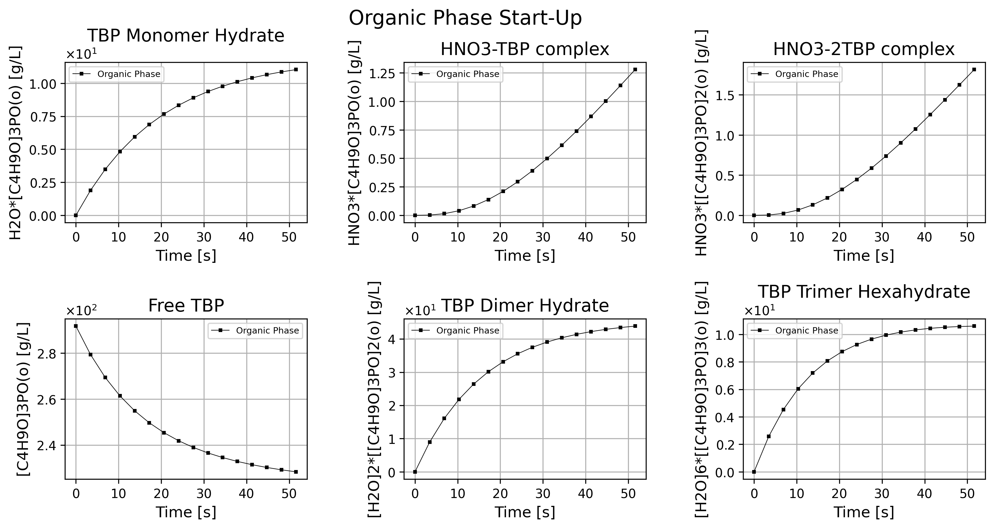
Figure 1: Organic phase species history dashboard at start-up.
, save_supporting_info=db_save, save_supporting_info=db_saveif cortix_ai:
    issues = '+ Title your reponse as: Overview of the Organic Phase Data at Start-Up.'
    cortix_ai.explain(phase=stg.organic_phase, issues=issues, markdown_header_level='<h4>', markdown_display=markdown_display, save_supporting_info=db_save)
Cortix AI assistant: working on explanation...
Overview of the Organic Phase Data at Start-Up.
Data summary (units: g/L unless noted)
Time: 0.000 → 51.604 s (data recorded at 16 time points).
[C₄H₉O]₃PO(o): 291.750 → 228.327 (monotonic decrease; loss ≈ 63.423 g/L).
H₂O·[C₄H₉O]₃PO(o): 0.000 → 11.032 (monotonic increase).
HNO₃·[C₄H₉O]₃PO(o): 0.000 → 1.27844 (small monotonic increase).
HNO₃·[[C₄H₉O]₃PO]₂(o): 0.000 → 1.81471 (small monotonic increase).
[H₂O]₂·[[C₄H₉O]₃PO]₂(o): 0.000 → 43.8774 (largest formed adduct by mass).
[H₂O]₆·[[C₄H₉O]₃PO]₃(o): 0.000 → 10.5998 (monotonic increase).
Mass balance and net changes
Total listed concentration at t = 0 s: 291.750 g/L (only [C₄H₉O]₃PO present).
Total listed concentration at t = 51.604 s: 296.929 g/L (sum of all columns).
Net change over 51.604 s: +5.179 g/L (~+1.78% of initial total).
Component-average rates (approximate):
[C₄H₉O]₃PO(o): −1.229 g·L⁻¹·s⁻¹ (loss).
Combined water-bearing adducts (H₂O· + [H₂O]₂· + [H₂O]₆·): +65.509 g·L⁻¹ total formed; average +1.269 g·L⁻¹·s⁻¹.
Combined HNO₃-bearing species: +3.093 g·L⁻¹ total formed; average +0.060 g·L⁻¹·s⁻¹.
Trends and relative magnitudes (descriptive)
The parent organic [C₄H₉O]₃PO(o) remains the dominant species at all times, though it steadily decreases from ~292 to ~228 g/L.
Water uptake is the principal transformation: most of the mass converted from the parent organic appears as water-containing adducts, especially [H₂O]₂·[[C₄H₉O]₃PO]₂(o), which reaches ~43.9 g/L.
Smaller but measurable formation of HNO₃-containing adducts occurs (combined ≈ 3.09 g/L by 51.6 s).
All newly formed species rise monotonically over the time series; no reversals or oscillations are present in the recorded interval.
Key observations
Rapid and monotonic conversion of the parent organic into water-bearing adducts is the dominant process in the 0–52 s window.
The largest single product by mass is [H₂O]₂·[[C₄H₉O]₃PO]₂(o); H₂O·[C₄H₉O]₃PO(o) and [H₂O]₆·[[C₄H₉O]₃PO]₃(o) are secondary contributors.
HNO₃ adducts form in small quantity compared with water adducts.
The total concentration of listed species increases slightly (~1.8%), indicating net uptake/formation (water and HNO₃ contributions exceed the loss of parent organic by ≈5.18 g/L over the recorded period).
AI Parameters:
+ LLM model (OpenAI) = gpt-5-mini
+ LLM cleverness     = 1.0
+ Total # of tokens  = 6438
'''Organic phase mass density'''
import matplotlib.pyplot as plt

quant = stg.mass_density_history('organic')

quant.plot(title='Organic Phase Mass Density @ %2.1f C Start-Up'%unit.convert_temperature(stg_temperature,
           'K','C'), x_scaling=1/stg.flow_residence_time_avg, x_label=r'Time [$\bar{\tau}$]', y_label=quant.latex_name+r'$-\rho_\text{diluent}$'
           ' ['+quant.unit+']', show=True, figsize=[10,3], error_data=False)

fig_count += 1
print(f'Figure {fig_count}: Organic phase mass density history at start-up.')
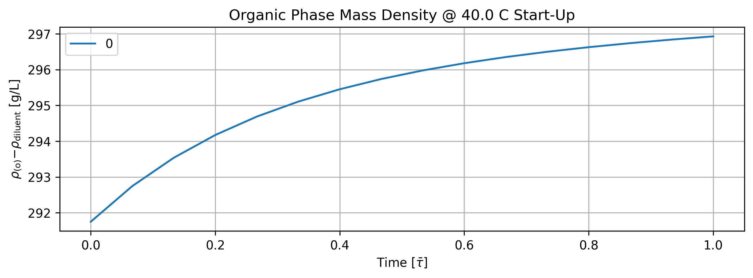
Figure 2: Organic phase mass density history at start-up.
tbl_count += 1
print(f'Table {tbl_count}: Organic phase mass density history at start-up.')
print('Time [s]  Organic Phase Mass Density [g/L]')
print(quant.value[::5].apply(lambda x: round(x,2)))
Table 1: Organic phase mass density history at start-up.
Time [s]  Organic Phase Mass Density [g/L]
0.000000     291.75
17.201342    295.11
34.402683    296.35
51.604025    296.93
Name: Organic Phase Mass Density [g/L]; Time History in [s], dtype: float64
1.5.2. Aqueous Phase Results#
'''Plot aqueous phase'''
# TODO: time axis normalized by phase flow residence time.
stg.aqueous_phase.plot(title='Aqueous Phase Start-Up', legend='Aqueous Phase', nrows=2,ncols=3, show=True, figsize=[12,6])

fig_count += 1
print(f'Figure {fig_count}: Aqueous phase species history dashboard at start-up.')
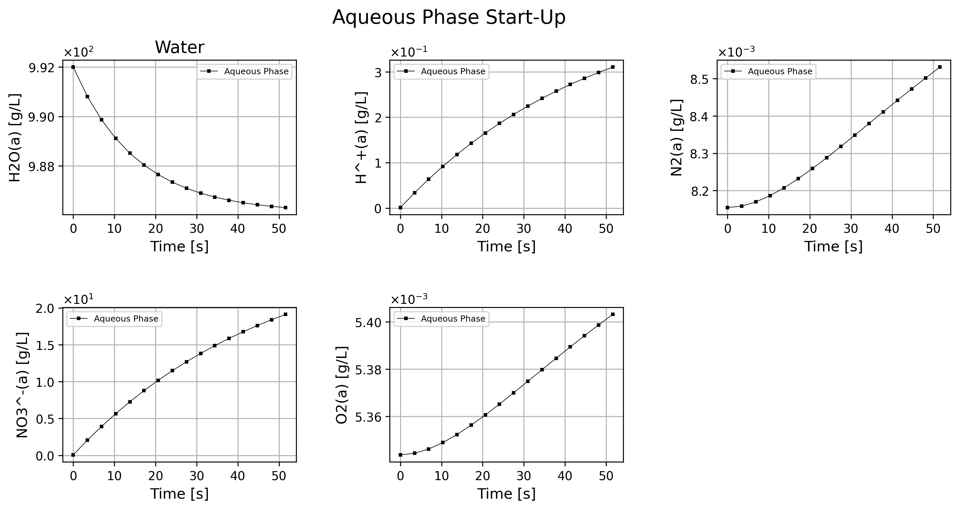
Figure 3: Aqueous phase species history dashboard at start-up.
if cortix_ai:
    issues = '+ Title your reponse as: Overview of the Aqueous Phase Data at Start-Up.'
    cortix_ai.explain(phase=stg.aqueous_phase, issues=issues, markdown_header_level='<h4>', markdown_display=markdown_display, save_supporting_info=db_save)
Cortix AI assistant: working on explanation...
Overview of the Aqueous Phase Data at Start-Up.
Quick numeric summary
Time span: 0 → 51.604 s (regular sampling interval ≈ 3.44027 s).
H₂O(a) [g/L]: 992 → 986.307; absolute change −5.693 g/L; mean rate −0.110 g·L⁻¹·s⁻¹; relative change ≈ −0.57%.
H⁺(a) [g/L]: 0.00100739 → 0.310391; absolute change +0.30938 g/L; mean rate +5.995×10⁻³ g·L⁻¹·s⁻¹; multiplicative change ≈ ×308.
N₂(a) [g/L]: 0.00815443 → 0.00853078; absolute change +3.76×10⁻⁴ g/L; mean rate +7.29×10⁻⁶ g·L⁻¹·s⁻¹; relative change ≈ +4.6%.
NO₃⁻(a) [g/L]: 0.0620055 → 19.1048; absolute change +19.0428 g/L; mean rate +0.3691 g·L⁻¹·s⁻¹; multiplicative change ≈ ×308.
O₂(a) [g/L]: 0.0053437 → 0.00540316; absolute change +5.95×10⁻⁵ g/L; mean rate +1.15×10⁻⁶ g·L⁻¹·s⁻¹; relative change ≈ +1.1%.
Trends and relationships
H⁺(a) and NO₃⁻(a) both rise monotonically and very steeply over the interval; their final/initial ratios are nearly identical (~308×), indicating proportional growth relative to their tiny initial concentrations.
H₂O(a) declines slowly and smoothly (small, steady loss ≈ 0.57%), while dissolved gases N₂(a) and O₂(a) remain nearly constant with only marginal increases.
In absolute mass terms, NO₃⁻(a) dominates the increases (≈19 g/L added), whereas H⁺(a) increases by ≈0.31 g/L; the large difference in absolute change reflects differing initial amounts and molar/gravimetric scales.
The time series is regularly sampled (constant step), supporting direct comparison of mean rates across species.
Observational notes and cautions
Because H⁺(a) and NO₃⁻(a) start from very small initial values, fold-change statistics are large; absolute-change and rate metrics give complementary perspective.
N₂(a) and O₂(a) show changes close to measurement/noise scale (10⁻⁴–10⁻⁵ g/L), so their small trends should be interpreted with caution unless sensor precision is known.
The large net increase in NO₃⁻(a) compared with the modest decrease in H₂O(a) implies addition/production of nitrate rather than simple conversion of bulk water into nitrate on a 1:1 mass basis.
Concise summary
Rapid onset of acidity and nitrate accumulation (H⁺(a) and NO₃⁻(a) rise sharply, ~×308), small steady depletion of water, and negligible changes in dissolved N₂ and O₂ over the first 51.6 s.
AI Parameters:
+ LLM model (OpenAI) = gpt-5-mini
+ LLM cleverness     = 1.0
+ Total # of tokens  = 6133
'''Aqueous phase mass density'''
import matplotlib.pyplot as plt

quant = stg.mass_density_history('aqueous')

quant.plot(title='Aqueous Phase Mass Density @ %2.1f C Start-Up'%unit.convert_temperature(stg_temperature,
           'K','C'), x_scaling=1/stg.flow_residence_time_avg, x_label=r'Time [$\bar{\tau}$]', y_label=quant.latex_name+
           ' ['+quant.unit+']', show=True, figsize=[10,3], error_data=False)

fig_count += 1
print(f'Figure {fig_count}: Aqueous phase mass density history at start-up.')
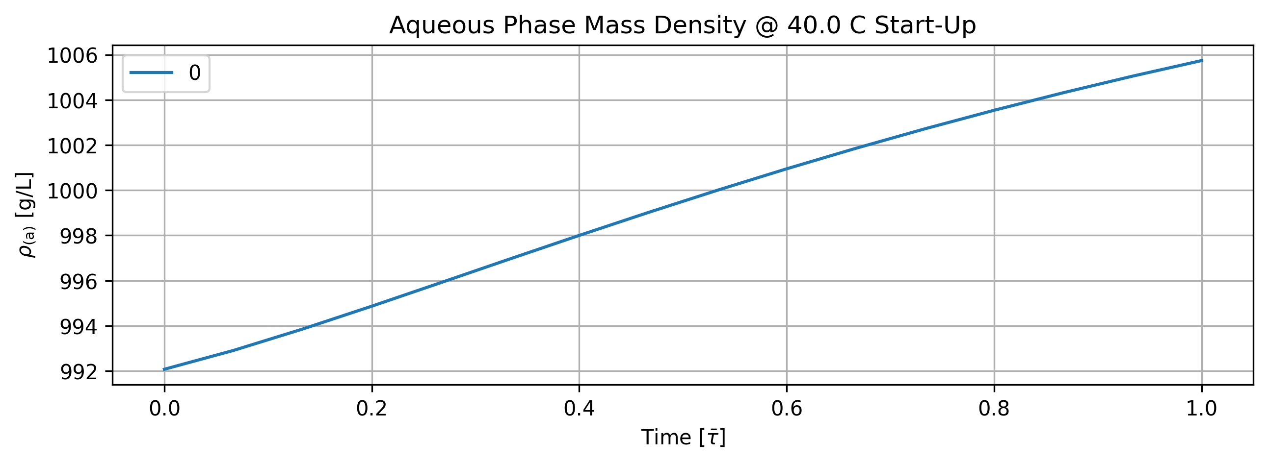
Figure 4: Aqueous phase mass density history at start-up.
tbl_count += 1
print(f'Table {tbl_count}: Aqueous phase mass density history at start-up.')
print('Time [s]  Aqueous Phase Mass Density [g/L]')
print(quant.value[::5].apply(lambda x: round(x,2)))
Table 2: Aqueous phase mass density history at start-up.
Time [s]  Aqueous Phase Mass Density [g/L]
0.000000      992.08
17.201342     996.96
34.402683    1001.85
51.604025    1005.74
Name: Aqueous Phase Mass Density [g/L]; Time History in [s], dtype: float64
1.5.3. Vapor Phase Results#
'''Plot vapor phase'''
# TODO: time axis normalized by phase flow residence time.
stg.vapor_phase.plot(title='Vapor Phase Start-Up', legend='Vapor Phase', nrows=2,ncols=3, show=True, figsize=[12,6])

fig_count += 1
print(f'Figure {fig_count}: Vapor phase species history dashboard start-up.')
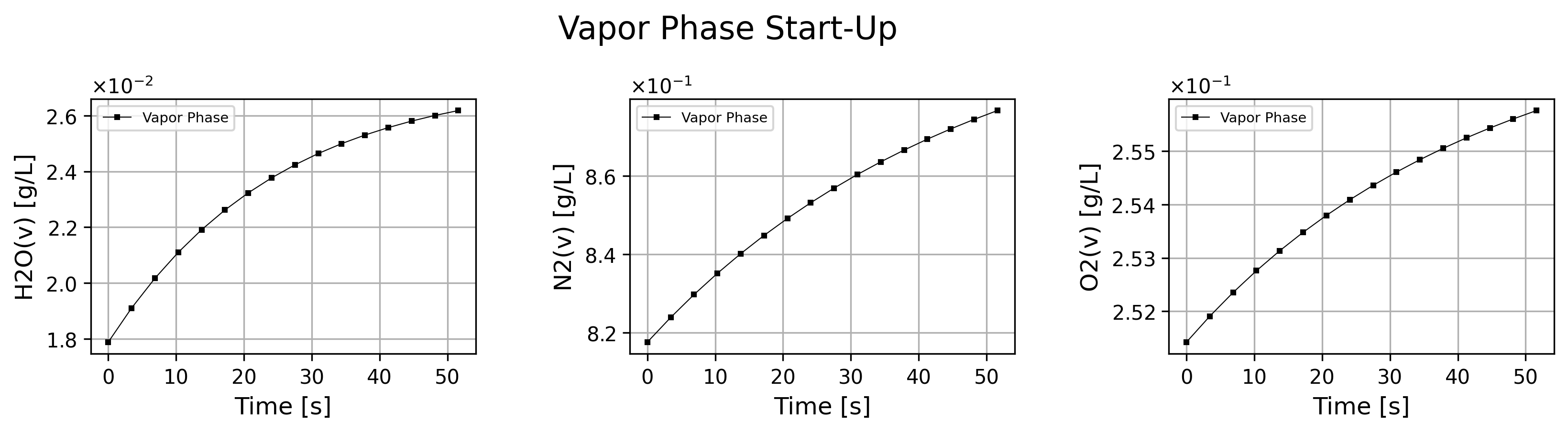
Figure 5: Vapor phase species history dashboard start-up.
if cortix_ai:
    issues = '+ Title your reponse as: Overview of the Vapor Phase Data at Start-Up.'
    cortix_ai.explain(phase=stg.vapor_phase, issues=issues, markdown_header_level='<h4>', markdown_display=markdown_display, save_supporting_info=db_save)
Cortix AI assistant: working on explanation...
Overview of the Vapor Phase Data at Start-Up
Summary
The table contains 16 time points from 0 to 51.604 s at regular increments (Δt = 3.44027 s).
All three vapor species — H₂O(v), N₂(v), and O₂(v) — increase monotonically over the measured interval.
Numeric summary (per species)
H₂O(v):
Min = 0.0178756 g/L, Max = 0.0261865 g/L, Range = 0.0083109 g/L.
Mean ≈ 0.0232840 g/L.
Absolute increase = 0.0083109 g/L over 51.604 s → average rate ≈ 1.61×10⁻⁴ g·L⁻¹·s⁻¹.
Relative increase ≈ 46.5% (largest relative change).
N₂(v):
Min = 0.817538 g/L, Max = 0.876683 g/L, Range = 0.059145 g/L.
Mean ≈ 0.8520755 g/L.
Absolute increase = 0.059145 g/L over 51.604 s → average rate ≈ 1.15×10⁻³ g·L⁻¹·s⁻¹.
Relative increase ≈ 7.23%.
O₂(v):
Min = 0.251420 g/L, Max = 0.255762 g/L, Range = 0.004342 g/L.
Mean ≈ 0.2539906 g/L.
Absolute increase = 0.004342 g/L over 51.604 s → average rate ≈ 8.41×10⁻⁵ g·L⁻¹·s⁻¹.
Relative increase ≈ 1.73% (smallest relative change).
Trends and comparisons
Temporal spacing: measurements are equally spaced (every 3.44027 s), enabling straightforward rate estimates by finite differences or linear fits.
Linearity / monotonicity: each concentration shows a smooth, monotonic rise across the interval; changes appear approximately linear on this short time scale.
Comparative rates: N₂ increases fastest in absolute terms (largest absolute slope), H₂O increases fastest in relative terms (largest percent change), and O₂ changes are the smallest both absolutely and relatively.
Magnitude ordering throughout the interval: N₂(v) >> O₂(v) > H₂O(v) (N₂ about an order of magnitude larger than O₂ and two orders larger than H₂O).
Concise interpretation
During start-up, the vapor composition shifts modestly: a notable fractional rise in H₂O concentration, a moderate absolute accumulation of N₂, and only a slight rise in O₂.
The data are consistent with a steady injection or release of N₂ and H₂O into the vapor phase, with O₂ remaining nearly constant relative to the others over the measured period.
AI Parameters:
+ LLM model (OpenAI) = gpt-5-mini
+ LLM cleverness     = 1.0
+ Total # of tokens  = 5397
'''Vapor phase mass density'''
import matplotlib.pyplot as plt

quant = stg.mass_density_history('vapor')

quant.plot(title='Vapor Phase Mass Density @ %2.1f C Start-Up'%unit.convert_temperature(stg_temperature,
           'K','C'), x_scaling=1/stg.flow_residence_time_avg, x_label=r'Time [$\bar{\tau}$]', y_label=quant.latex_name+
           ' ['+quant.unit+']', show=True, figsize=[10,3], error_data=False)

fig_count += 1
print(f'Figure {fig_count}: Vapor phase mass density history at start-up.')
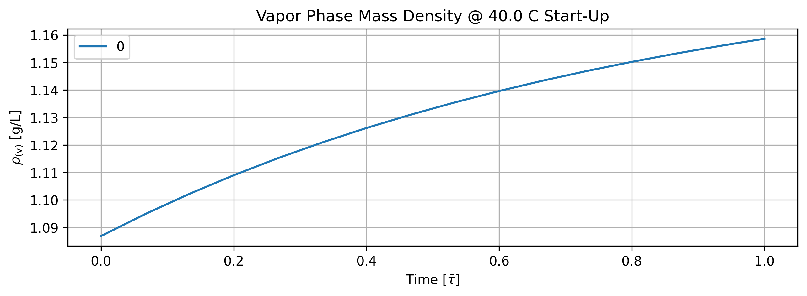
Figure 6: Vapor phase mass density history at start-up.
tbl_count += 1
print(f'Table {tbl_count}: Vapor phase mass density history at start-up.')
print('Time [s]  Vapor Phase Mass Density [g/L]')
print(quant.value[::5].apply(lambda x: round(x,2)))
Table 3: Vapor phase mass density history at start-up.
Time [s]  Vapor Phase Mass Density [g/L]
0.000000     1.09
17.201342    1.12
34.402683    1.14
51.604025    1.16
Name: Vapor Phase Mass Density [g/L]; Time History in [s], dtype: float64
1.5.3.1. Relative Humidity#
'''Compute relative humidity in the vapor phase'''
import matplotlib.pyplot as plt
from solvex import air_relative_humidity
from copy import deepcopy

h2o_vap_pd_series = deepcopy(stg.vapor_phase.df['H2O(v)'])
for idx, rho_h2o in enumerate(h2o_vap_pd_series):
    h2o_vap_pd_series.iloc[idx] = air_relative_humidity(stg_temperature, rho_h2o)
rh_pd_series = h2o_vap_pd_series
time_unit = stg.vapor_phase.time_unit
rh_pd_series.name = f'Relative Humidity History [{time_unit}]'

quant = Quantity(name=rh_pd_series.name, latex_name='RH', unit='%', info=f'Relative Humidity History (Vapor Phase) [{time_unit}]')
quant.value = h2o_vap_pd_series
quant.plot(title='Stage Rel. Humidity @ %2.1f C Start-Up'%unit.convert_temperature(stg_temperature, 'K','C'),
           x_scaling=1/stg.flow_residence_time_avg, x_label=r'Time [$\bar{\tau}$]', y_label=quant.latex_name+' ['+quant.unit+']', show=True,
           figsize=[10,3])

fig_count += 1
print(f'Figure {fig_count}: Stage relative humidity history at start-up.')
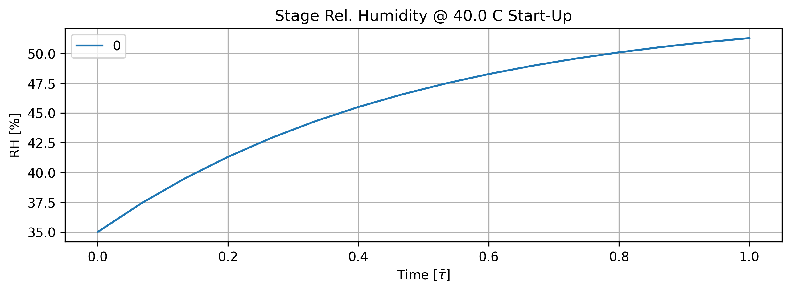
Figure 7: Stage relative humidity history at start-up.
tbl_count += 1
print(f'Table {tbl_count}: Stage relative humidity history at start-up.')
print('Time [s]  Rel. Humidity [%]')
print(quant.value[::5].apply(lambda x: round(x,2)))
Table 4: Stage relative humidity history at start-up.
Time [s]  Rel. Humidity [%]
0.000000     35.00
17.201342    44.28
34.402683    48.95
51.604025    51.27
Name: Relative Humidity History [s], dtype: float64
if cortix_ai:
    issues = '+ Title your reponse as: Overview of the Relative Humidity Data at Start-Up.'
    cortix_ai.explain(quant=quant, issues=issues, markdown_header_level='<h5>', markdown_display=markdown_display, save_supporting_info=db_save)
Cortix AI assistant: working on explanation...
Overview of the Relative Humidity Data at Start-Up.
Dataset and labels
Time is given in seconds (0 to 48.1638 s). Relative Humidity History (vapor phase) is given in percent [%].
Eight measurements sampled starting at t = 0 s; sample-to-sample interval is uniform (≈ 6.88054 s).
Basic behaviour and trend
Relative humidity rises monotonically from 35.0000% to 50.9284% over the recorded interval.
The increase decelerates with time (larger %/s near the start, smaller %/s later), indicating a saturating approach toward a steady value near ≈51%.
Global summary statistics
Minimum: 35.0000%
Maximum: 50.9284%
Total change (ΔRH): 15.9284%
Mean (arithmetic): 45.0359%
Median: 46.4743%
Sample standard deviation: ≈ 5.58%
Total duration: 48.1638 s
Average rate over entire period: 15.9284% / 48.1638 s ≈ 0.3307 %/s
Sampling characteristics
Nominal sampling interval: ≈ 6.88054 s (uniform between rows).
Equivalent sampling frequency: ≈ 0.1453 Hz (1/6.88054).
Interval-by-interval changes (each interval ≈ 6.8805 s)
t 0.0000 -> 6.8805 s: ΔRH = +4.4868% → rate ≈ 0.6523 %/s
t 6.8805 -> 13.7611 s: ΔRH = +3.4119% → rate ≈ 0.4961 %/s
t 13.7611 -> 20.6416 s: ΔRH = +2.5921% → rate ≈ 0.3767 %/s
t 20.6416 -> 27.5221 s: ΔRH = +1.9669% → rate ≈ 0.2858 %/s
t 27.5221 -> 34.4027 s: ΔRH = +1.4906% → rate ≈ 0.2167 %/s
t 34.4027 -> 41.2832 s: ΔRH = +1.1280% → rate ≈ 0.1639 %/s
t 41.2832 -> 48.1638 s: ΔRH = +0.8521% → rate ≈ 0.1239 %/s
Key observations (concise)
The RH rises steadily and monotonically; every sampled point is higher than the previous.
The per-interval rate decreases monotonically, consistent with a first-order (exponential-like) approach to an asymptote near 51%.
Sampling is regular and dense enough (≈ 6.9 s spacing) to resolve the deceleration in the RH increase over the recorded 48 s.
AI Parameters:
+ LLM model (OpenAI) = gpt-5-mini
+ LLM cleverness     = 1.0
+ Total # of tokens  = 4742
1.5.4. Overall Stage Efficiency#
Stage efficiency measures how close to chemical equilibrium the system is as a whole. This is a direct result of the reaction relaxation time which is dependent on the mass transfer coefficients of the system. Much more needs to be investigated in this project with various degrees of theory but these results represent the beginning of a solid development.
'''Stage overall efficiency'''

quant = stg.efficiency_history(mean=True)
quant.plot(title='Stage Efficiency @ %2.1f C Start-Up'%unit.convert_temperature(stg_temperature,
           'K','C'), x_scaling=1/stg.flow_residence_time_avg, x_label=r'Time [$\bar{\tau}$]', y_label=quant.latex_name+
           ' ['+quant.unit+']', show=True, figsize=[10,3], error_data=True)

fig_count += 1
print(f'Figure {fig_count}: Stage efficiency history at start-up.')
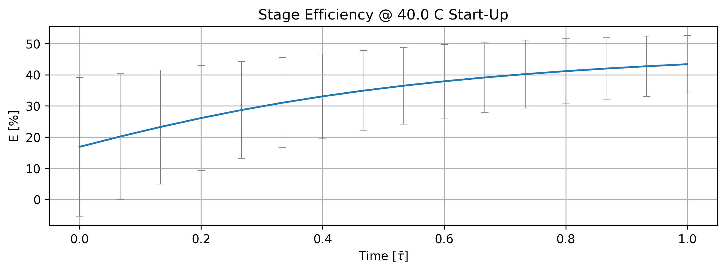
Figure 8: Stage efficiency history at start-up.
tbl_count += 1
print(f'Table {tbl_count}: Stage efficiency history at start-up.')
print('Time [s]  (Stage. Eff., +-std) [%]')
time_name = ''
import pandas as pd
df = (quant.value.apply(pd.Series).mul(1)
       .rename(index=lambda i: round(i/unit.min,2))
       .set_axis(['',''], axis=1).rename_axis(time_name)
       .round(3))
print(df.to_string(max_rows=20, min_rows=20))
Table 5: Stage efficiency history at start-up.
Time [s]  (Stage. Eff., +-std) [%]


0.00  16.875  22.212
0.06  20.172  20.127
0.11  23.258  18.305
0.17  26.106  16.757
0.23  28.693  15.478
0.29  31.001  14.440
0.34  33.063  13.593
0.40  34.884  12.895
0.46  36.484  12.303
0.52  37.888  11.783
0.57  39.118  11.309
0.63  40.197  10.864
0.69  41.144  10.437
0.75  41.978  10.022
0.80  42.715   9.614
0.86  43.368   9.213
if cortix_ai:
    issues = '+ Title your reponse as: Overview of the Stage Efficiency Data at Start-Up.'
    cortix_ai.explain(quant=quant, issues=issues, markdown_header_level='<h4>', markdown_display=markdown_display, print_prompt=False, save_supporting_info=db_save)
Cortix AI assistant: working on explanation...
Overview of the Stage Efficiency Data at Start-Up
Data structure and units
The table contains 8 time-sampled records (index 0..7).
time [s]: evenly spaced samples every 6.88054 s (0 → 48.1638 s).
Columns “0” and “1”: stage efficiencies in percent (%) given as mean values (the table header indicates “mean, +/- std” but no ± values are present in the cells).
Statistical summary (per stage, sample standard deviation)
Stage 0: mean = 32.67% ; sample standard deviation ≈ 9.12%.
Stage 1: mean = 14.16% ; sample standard deviation ≈ 4.31%.
Range and extrema
Stage 0: min = 16.8752% at t = 0 s, max = 42.7149% at t = 48.1638 s, total change = +25.8397%.
Stage 1: max = 22.2119% at t = 0 s, min = 9.61383% at t = 48.1638 s, total change = −12.59807%.
Temporal trends and rates
Sampling is uniform (Δt = 6.88054 s).
Stage 0 exhibits a clear monotonic increase across the record.
Average rate of change ≈ +0.537 %/s (25.8397% / 48.1638 s).
Stage 1 exhibits a clear monotonic decrease across the record.
Average rate of change ≈ −0.262 %/s (−12.59807% / 48.1638 s).
Observations and implications
The two stages move in opposite directions: Stage 0 efficiency increases during start-up while Stage 1 efficiency decreases.
Stage 0 shows larger absolute variability (higher mean and larger standard deviation) than Stage 1 over the sampled interval.
The header’s mention of “± std” is not reflected in the table cells; only mean values are provided.
AI Parameters:
+ LLM model (OpenAI) = gpt-5-mini
+ LLM cleverness     = 1.0
+ Total # of tokens  = 4735
'''Individual reaction efficiency'''

quant = stg.efficiency_history()
quant.plot(title='Reaction Efficiency @ %2.1f C Start-Up'%unit.convert_temperature(stg_temperature,
           'K','C'), x_scaling=1/stg.flow_residence_time_avg, x_label=r'Time [$\bar{\tau}$]', y_label=quant.latex_name+
           ' ['+quant.unit+']', legend=stg.rxn_mech.reactions, show=True, figsize=[10,3])

fig_count += 1
print(f'Figure {fig_count}: Reaction efficiency history at start-up.')
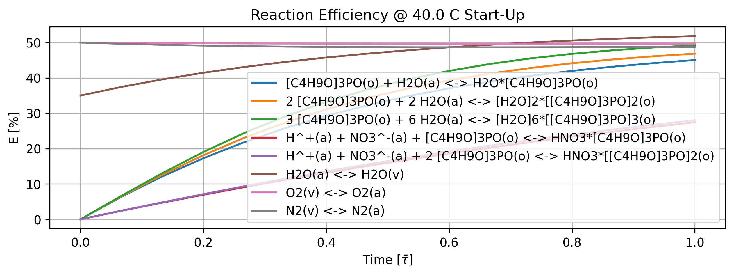
Figure 9: Reaction efficiency history at start-up.
'''Individual reaction efficiency'''

quant = stg.efficiency_history()

tbl_count += 1
print(f'Table {tbl_count}: Reaction efficiency history at start-up.')
print('Time [min]    Rxn Eff. [%]')

col_names = [f'r{i}' for i in range(len(stg.rxn_mech.reactions))]
time_name = ''
df = (quant.value.apply(pd.Series).mul(1)
       .rename(index=lambda i: round(i/unit.min,2))
       .set_axis(col_names, axis=1).rename_axis(time_name)
       .round(3))
print(df.to_string(max_rows=20, min_rows=20))
Table 6: Reaction efficiency history at start-up.
Time [min]    Rxn Eff. [%]
          r0      r1      r2      r3      r4      r5      r6      r7

0.00   0.000   0.000   0.000   0.000   0.000  35.002  50.000  50.000
0.06   6.372   6.506   6.645   2.416   2.443  37.442  49.910  49.642
0.11  12.132  12.583  13.058   4.712   4.802  39.578  49.839  49.359
0.17  17.274  18.119  19.025   6.943   7.114  41.447  49.783  49.140
0.23  21.816  23.063  24.417   9.099   9.356  43.082  49.741  48.972
0.29  25.784  27.351  29.114  11.174  11.512  44.513  49.710  48.847
0.34  29.247  31.098  33.208  13.165  13.576  45.763  49.688  48.758
0.40  32.244  34.304  36.682  15.069  15.541  46.857  49.674  48.698
0.46  34.829  37.023  39.587  16.889  17.409  47.813  49.665  48.661
0.52  37.050  39.311  41.987  18.625  19.180  48.648  49.661  48.644
0.57  38.954  41.224  43.947  20.280  20.860  49.377  49.662  48.643
0.63  40.584  42.817  45.533  21.858  22.451  50.014  49.665  48.654
0.69  41.977  44.136  46.803  23.361  23.960  50.571  49.671  48.675
0.75  43.167  45.226  47.811  24.793  25.390  51.056  49.678  48.704
0.80  44.183  46.123  48.604  26.156  26.746  51.480  49.688  48.739
0.86  45.050  46.860  49.221  27.454  28.032  51.850  49.698  48.779
if cortix_ai:
    issues = '+ Title your reponse as: Overview of Individual Reaction Efficiency at Start-Up.'
    cortix_ai.explain(quant=quant, issues=issues, markdown_header_level='<h4>', markdown_display=markdown_display, print_prompt=False, save_supporting_info=db_save)
Cortix AI assistant: working on explanation...
Overview of Individual Reaction Efficiency at Start-Up
Summary of overall behaviour:
Reactions 0–2 (hydrated adduct formation of [C4H9O]3PO) start at 0% and increase monotonically over the 48.16 s window, reaching roughly 44% (rxn 0), 46% (rxn 1) and 48.6% (rxn 2) by the last time point.
Reactions 3–4 (HNO3 adduct formation) also start at 0% and rise steadily but remain substantially lower than the hydration series, ending near 26% (rxn 3) and 26.7% (rxn 4).
Reaction 5 (H2O(a) <-> H2O(v)) starts nonzero (35.00%) and increases to ~51.48%, crossing 50% during the interval.
Reactions 6 and 7 (O2 and N2 gas–aerosol exchange) start at 50% and remain essentially constant around 49.6–49.8% (O2) and ~48.6–49.0% (N2), showing only small fluctuations.
Per-reaction details (indexed to the supplied ordered reactions list):
0 — [C4H9O]3PO(o) + H2O(a) <-> H2O*[C4H9O]3PO(o): 0% at t=0 → 44.1833% at t=48.1638 s. Monotonic rise, fairly rapid initially and slowing toward ~44–45%.
1 — 2 [C4H9O]3PO(o) + 2 H2O(a) <-> [H2O]2*[[C4H9O]3PO]2(o): 0% → 46.1232% over the same interval. Similar shape to rxn 0 but reaches a slightly higher efficiency.
2 — 3 [C4H9O]3PO(o) + 6 H2O(a) <-> [H2O]6*[[C4H9O]3PO]3(o): 0% → 48.6038%. Fastest rise among the hydration series and highest final efficiency of the three.
3 — H^+(a) + NO3^-(a) + [C4H9O]3PO(o) <-> HNO3*[C4H9O]3PO(o): 0% → 26.1560%. Steady increase but remaining substantially below hydration efficiencies.
4 — H^+(a) + NO3^-(a) + 2 [C4H9O]3PO(o) <-> HNO3*[[C4H9O]3PO]2(o): 0% → 26.7457%. Very similar time history and magnitude to rxn 3.
5 — H2O(a) <-> H2O(v): 35.0016% at t=0 → 51.4802% at t=48.1638 s. Begins already active and crosses 50%, showing the largest absolute increase among all reactions (~16.5 percentage points).
6 — O2(v) <-> O2(a): 50.0000% at t=0 → ~49.68% (fluctuating 49.66–49.84%) thereafter. Effectively steady around ~49.7%.
7 — N2(v) <-> N2(a): 50.0000% at t=0 → ~48.74% at final time (lowest point ~48.64%). Small net decrease from initial 50%, then slight recovery.
Key observations and implications:
The three multi-water adduct formation reactions (0–2) progress from zero toward similar mid-to-high efficiencies, with larger complexes (rxn 2) achieving the highest efficiency by 48 s.
The two HNO3 adduct reactions (3–4) follow the same qualitative trend but plateau at much lower efficiencies (~26–27%).
The H2O phase exchange (rxn 5) is active at start-up and becomes the most efficient single process by the end of the window, exceeding 50%.
Gas–aerosol exchanges for O2 and N2 (6–7) are essentially at steady-state near 49–50% for the whole interval, indicating they are equilibrated from t=0 with only small adjustments.
AI Parameters:
+ LLM model (OpenAI) = gpt-5-mini
+ LLM cleverness     = 1.0
+ Total # of tokens  = 5460
1.5.5. Reaction Rate Density#
This quantity only makes sense per volume of the mixture.
'''Reaction rate density'''
import matplotlib.pyplot as plt

quant = stg.r_vec_history() # mole/m^3-s

quant.plot(title='Reaction Rate Density @ %2.1f C Start-Up'%unit.convert_temperature(stg_temperature,
           'K','C'), x_scaling=1/stg.flow_residence_time_avg, x_label=r'Time [$\bar{\tau}$]', y_label=quant.latex_name+
           ' ['+quant.unit+']', legend=stg.rxn_mech.reactions, show=True, figsize=[10,3], error_data=False)

fig_count += 1
print(f'Figure {fig_count}: Reaction rate density history at start-up.')
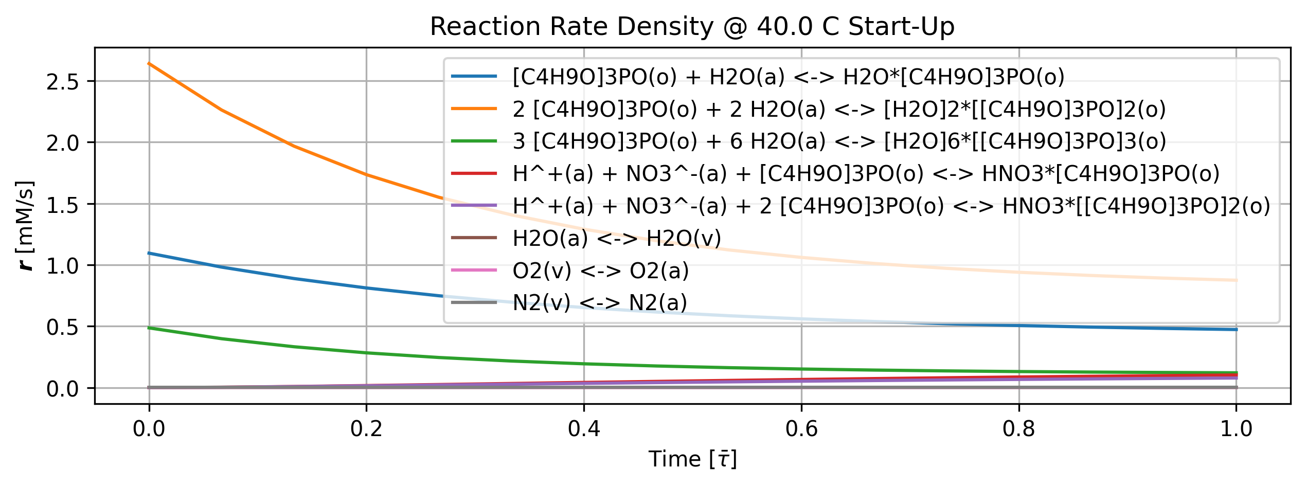
Figure 10: Reaction rate density history at start-up.
tbl_count += 1
print(f'Table {tbl_count}: Reaction rate density history at start-up.')
print('Time [min]      r [mM/s]')
import pandas as pd
col_names = [f'r{i}' for i in range(len(stg.rxn_mech.reactions))]
time_name = 't [min]'
df = (quant.value.apply(pd.Series).mul(1)
       .rename(index=lambda i: round(i/unit.min,2))
       .set_axis(col_names, axis=1).rename_axis(time_name)
       .round(4))
print(df.to_string(max_rows=20, min_rows=20))
Table 7: Reaction rate density history at start-up.
Time [min]      r [mM/s]
             r0      r1      r2      r3      r4      r5      r6      r7
t [min]
0.00     1.0955  2.6403  0.4865  0.0000  0.0000  0.0019  0.0014  0.0024
0.06     0.9820  2.2625  0.3985  0.0029  0.0028  0.0019  0.0014  0.0025
0.11     0.8888  1.9675  0.3329  0.0089  0.0081  0.0018  0.0014  0.0025
0.17     0.8119  1.7352  0.2832  0.0165  0.0145  0.0017  0.0014  0.0025
0.23     0.7484  1.5508  0.2453  0.0248  0.0212  0.0017  0.0014  0.0025
0.29     0.6961  1.4077  0.2166  0.0334  0.0280  0.0016  0.0014  0.0026
0.34     0.6524  1.2909  0.1939  0.0420  0.0345  0.0016  0.0014  0.0026
0.40     0.6160  1.1972  0.1762  0.0504  0.0408  0.0016  0.0014  0.0026
0.46     0.5856  1.1218  0.1624  0.0585  0.0467  0.0015  0.0014  0.0026
0.52     0.5601  1.0610  0.1515  0.0662  0.0523  0.0015  0.0014  0.0026
0.57     0.5388  1.0118  0.1429  0.0734  0.0575  0.0015  0.0014  0.0026
0.63     0.5209  0.9721  0.1362  0.0802  0.0624  0.0015  0.0014  0.0026
0.69     0.5058  0.9398  0.1308  0.0865  0.0668  0.0015  0.0014  0.0026
0.75     0.4931  0.9136  0.1266  0.0923  0.0710  0.0014  0.0014  0.0027
0.80     0.4824  0.8923  0.1232  0.0977  0.0747  0.0014  0.0014  0.0027
0.86     0.4733  0.8750  0.1206  0.1026  0.0782  0.0014  0.0014  0.0027
if cortix_ai:
    issues = '+ Title your reponse as: Overview of Reaction Rates Density at Start-Up.'
    cortix_ai.explain(quant=quant, issues=issues, markdown_header_level='<h4>', markdown_display=markdown_display, print_prompt=False, save_supporting_info=db_save)
Cortix AI assistant: working on explanation...
Overview of Reaction Rates Density at Start-Up.
This response summarizes the time history (0 → 48.1638 s) of reaction-rate densities (units: mM/s) for the eight ordered reactions provided. Times are sampled every 6.88054 s (8 points). The columns 0–7 map to the reactions in the given order (converted to the requested chemical formatting).
Key points
The three leftmost reactions (columns 0–2) exhibit large absolute rates (0.1–2.6 mM/s) and decline monotonically over the recorded period.
Two intermediate reactions (columns 3–4) start effectively at micro-magnitude rates and grow by many orders of magnitude to reach ~0.098 and ~0.075 mM/s; their growth rate slows with time.
The three rightmost reactions (columns 5–7) remain small (<3×10⁻³ mM/s), with modest relative changes (±≈25% or less).
Time spacing is uniform: Δt = 6.88054 s; total span ≈ 48.16 s.
Column → reaction mapping (formatted)
Column 0: [C4H9O]₃PO(o) + H₂O(a) <-> H₂O·[C4H9O]₃PO(o)
Column 1: 2 [C4H9O]₃PO(o) + 2 H₂O(a) <-> [H₂O]₂·[[C4H9O]₃PO]₂(o)
Column 2: 3 [C4H9O]₃PO(o) + 6 H₂O(a) <-> [H₂O]₆·[[C4H9O]₃PO]₃(o)
Column 3: H⁺(a) + NO₃⁻(a) + [C4H9O]₃PO(o) <-> HNO₃·[C4H9O]₃PO(o)
Column 4: H⁺(a) + NO₃⁻(a) + 2 [C4H9O]₃PO(o) <-> HNO₃·[[C4H9O]₃PO]₂(o)
Column 5: H₂O(a) <-> H₂O(v)
Column 6: O₂(v) <-> O₂(a)
Column 7: N₂(v) <-> N₂(a)
Per-reaction quantitative trends (t = 0 → 48.1638 s)
Column 0: 1.09551 → 0.482355 mM/s (decrease ≈ −56.0%); large initial rate, monotonic decline.
Column 1: 2.64031 → 0.892309 mM/s (decrease ≈ −66.2%); largest initial rate, marked decline.
Column 2: 0.486462 → 0.123215 mM/s (decrease ≈ −74.7%); substantial fractional drop.
Column 3: 5.38343×10⁻⁶ → 0.0976534 mM/s (absolute increase ≈ +0.09765 mM/s); growth by many orders of magnitude, with incremental growth slowing at later times.
Column 4: 5.28724×10⁻⁶ → 0.0747478 mM/s (absolute increase ≈ +0.07474 mM/s); similar pattern to column 3 but lower final magnitude.
Column 5: 0.00192554 → 0.00142203 mM/s (decrease ≈ −26.1%); small magnitude, modest decline.
Column 6: 0.00139164 → 0.00142364 mM/s (increase ≈ +2.3%); essentially steady at ~1.4×10⁻³ mM/s.
Column 7: 0.00242574 → 0.00265994 mM/s (increase ≈ +9.7%); small magnitude, slight upward trend.
Global interpretation
Massively active processes are the first three reactions (columns 0–2); their declining rates suggest depletion of reactant availability or approach toward a slower regime over the 48 s window.
The nitric-acid–adduct formation reactions (columns 3–4) transition from negligible to measurable rates, indicating rapid onset of those pathways during start-up; their growth decelerates by the final samples.
Gas–liquid exchange and pure water vaporization/condensation reactions (columns 5–7) remain minor in magnitude compared with organophosphorus hydration/aggregation and acid-adduct formation, with column 6 near-constant and columns 5 and 7 changing only modestly.
By t ≈ 48 s the system shows clear trends but not full convergence to a single steady-state for all reactions: columns 0–2 still have notable slopes and columns 3–4 are still increasing, though their growth rate is slowing.
AI Parameters:
+ LLM model (OpenAI) = gpt-5-mini
+ LLM cleverness     = 1.0
+ Total # of tokens  = 7257
1.5.6. Species Generation Rate Density#
This quantity is on the basis of mixing volume so all species generation values can be compared.
'''Species generation rate density'''
import matplotlib.pyplot as plt

quant = stg.g_vec_history() # mole/m^3-s

quant.plot(title='Species Generation Rate Density @ %2.1f C Start-Up'%unit.convert_temperature(stg_temperature,
           'K','C'), x_scaling=1/stg.flow_residence_time_avg, x_label=r'Time [$\bar{\tau}$]', y_label=quant.latex_name+
           ' ['+quant.unit+']', legend=stg.rxn_mech.species_names, show=True, figsize=[10,3], error_data=False)

fig_count += 1
print(f'Figure {fig_count}: Species generation rate density history at start-up.')
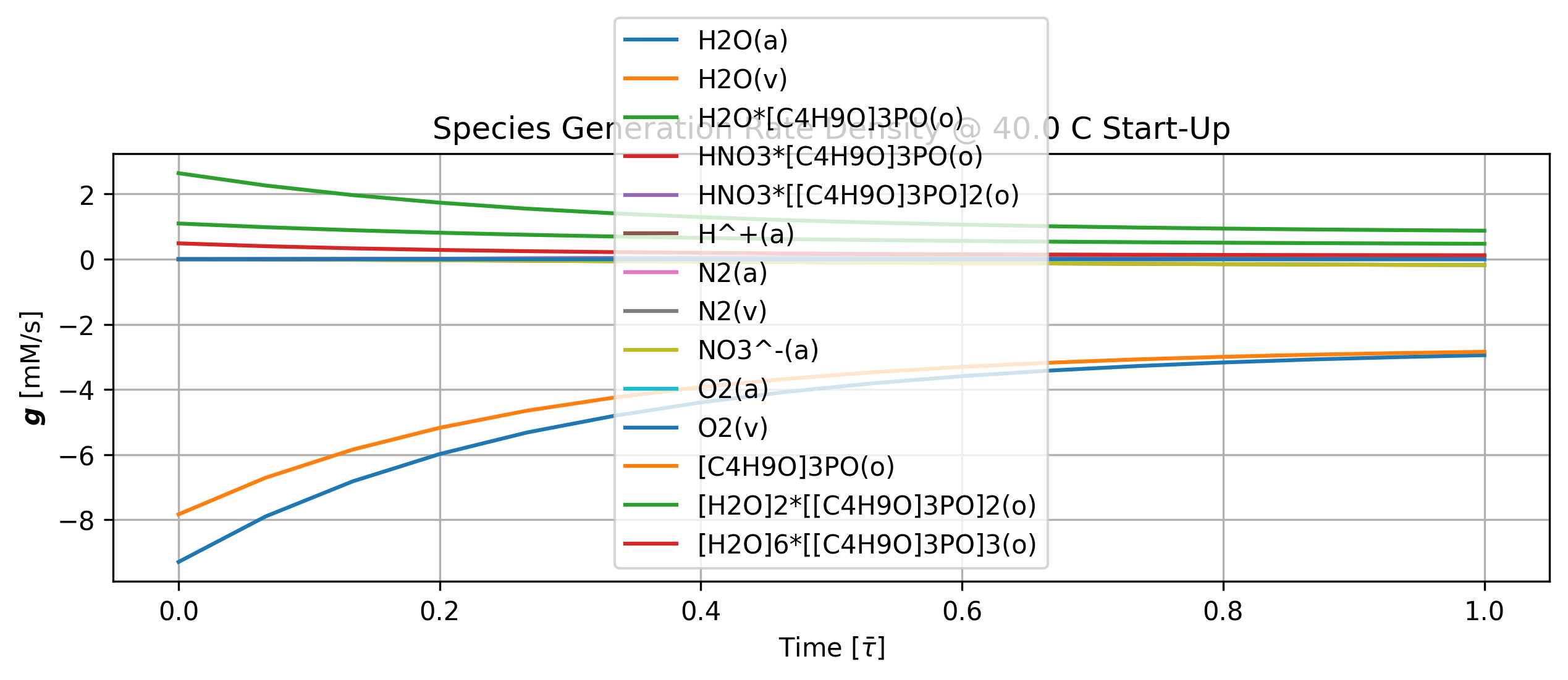
Figure 11: Species generation rate density history at start-up.
tbl_count += 1
print(f'Table {tbl_count}: Species generation rate density history at start-up.')
print('Time [min]        g [mM/s]')
import pandas as pd
col_names = [f'a{i}' for i in range(len(stg.rxn_mech.species_names))]
time_name = 't [min]'
df = (quant.value.apply(pd.Series).mul(1)
       .rename(index=lambda i: round(i/unit.min,2))
       .set_axis(col_names, axis=1).rename_axis(time_name)
       .round(4))
print(df.to_string(max_rows=20, min_rows=20))
Table 8: Species generation rate density history at start-up.
Time [min]        g [mM/s]
             a0      a1      a2      a3      a4      a5      a6      a7      a8      a9     a10     a11     a12     a13
t [min]
0.00    -9.2968  0.0019  1.0955  0.0000  0.0000 -0.0000  0.0024 -0.0024 -0.0000  0.0014 -0.0014 -7.8355  2.6403  0.4865
0.06    -7.8999  0.0019  0.9820  0.0029  0.0028 -0.0057  0.0025 -0.0025 -0.0057  0.0014 -0.0014 -6.7110  2.2625  0.3985
0.11    -6.8229  0.0018  0.8888  0.0089  0.0081 -0.0170  0.0025 -0.0025 -0.0170  0.0014 -0.0014 -5.8476  1.9675  0.3329
0.17    -5.9834  0.0017  0.8119  0.0165  0.0145 -0.0310  0.0025 -0.0025 -0.0310  0.0014 -0.0014 -5.1775  1.7352  0.2832
0.23    -5.3232  0.0017  0.7484  0.0248  0.0212 -0.0461  0.0025 -0.0025 -0.0461  0.0014 -0.0014 -4.6531  1.5508  0.2453
0.29    -4.8125  0.0016  0.6961  0.0334  0.0280 -0.0614  0.0026 -0.0026 -0.0614  0.0014 -0.0014 -4.2506  1.4077  0.2166
0.34    -4.3992  0.0016  0.6524  0.0420  0.0345 -0.0766  0.0026 -0.0026 -0.0766  0.0014 -0.0014 -3.9270  1.2909  0.1939
0.40    -4.0693  0.0016  0.6160  0.0504  0.0408 -0.0912  0.0026 -0.0026 -0.0912  0.0014 -0.0014 -3.6711  1.1972  0.1762
0.46    -3.8050  0.0015  0.5856  0.0585  0.0467 -0.1052  0.0026 -0.0026 -0.1052  0.0014 -0.0014 -3.4683  1.1218  0.1624
0.52    -3.5926  0.0015  0.5601  0.0662  0.0523 -0.1185  0.0026 -0.0026 -0.1185  0.0014 -0.0014 -3.3074  1.0610  0.1515
0.57    -3.4215  0.0015  0.5388  0.0734  0.0575 -0.1309  0.0026 -0.0026 -0.1309  0.0014 -0.0014 -3.1797  1.0118  0.1429
0.63    -3.2834  0.0015  0.5209  0.0802  0.0624 -0.1425  0.0026 -0.0026 -0.1425  0.0014 -0.0014 -3.0783  0.9721  0.1362
0.69    -3.1717  0.0015  0.5058  0.0865  0.0668 -0.1533  0.0026 -0.0026 -0.1533  0.0014 -0.0014 -2.9979  0.9398  0.1308
0.75    -3.0811  0.0014  0.4931  0.0923  0.0710 -0.1632  0.0027 -0.0027 -0.1632  0.0014 -0.0014 -2.9342  0.9136  0.1266
0.80    -3.0077  0.0014  0.4824  0.0977  0.0747 -0.1724  0.0027 -0.0027 -0.1724  0.0014 -0.0014 -2.8838  0.8923  0.1232
0.86    -2.9480  0.0014  0.4733  0.1026  0.0782 -0.1808  0.0027 -0.0027 -0.1808  0.0014 -0.0014 -2.8439  0.8750  0.1206
'''Produced species generation rate density'''
import matplotlib.pyplot as plt

ids, quant_produced = stg.g_vec_history(produced=True) # mole/m^3-s

quant_produced.plot(title='Produced Species Generation Rate Density @ %2.1f C Start-Up'%unit.convert_temperature(stg_temperature,
           'K','C'), x_scaling=1/stg.flow_residence_time_avg, x_label=r'Time [$\bar{\tau}$]', y_label=quant.latex_name+
           ' ['+quant_produced.unit+']', legend=list(np.array(stg.rxn_mech.species_names)[ids]), show=True, figsize=[10,3], error_data=False)

fig_count += 1
print(f'Figure {fig_count}: Produced species generation rate density history at start-up.')
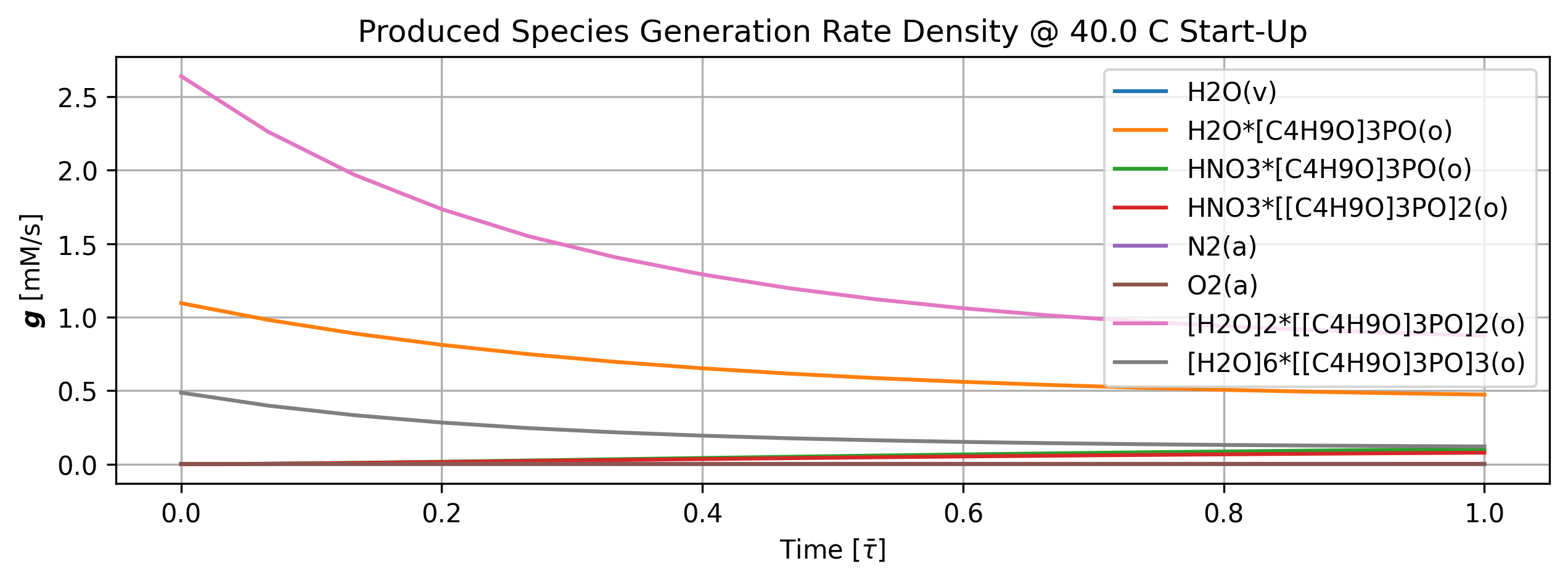
Figure 12: Produced species generation rate density history at start-up.
if cortix_ai:
    issues = '+ Title your reponse as: Overview of Species Generation Rates Density at Start-Up.'
    cortix_ai.explain(quant=quant, issues=issues, markdown_header_level='<h4>', markdown_display=markdown_display, print_prompt=False, save_supporting_info=db_save)
Cortix AI assistant: working on explanation...
Overview of Species Generation Rates Density at Start-Up.
Summary
The table gives species generation-rate densities (mM/s) for 14 ordered species at 8 time points (0 s through 48.1638 s). Most species show smooth, monotonic trends (either increasing or decreasing) over the provided start-up interval. Magnitudes span from ~10⁻⁶–10⁻³ mM/s for trace gas/vibrational modes up to several mM/s for condensed-phase species.
Per-species time behavior
H₂O(a): negative throughout, from −9.29682 at 0 s to −3.00768 at 48.1638 s; magnitude decreases (becomes less negative) monotonically (consumption diminishing with time).
H₂O(v): small positive rates, slowly decreasing from 0.00192554 to 0.00142203 mM/s (gentle monotonic decline).
H₂O*[C₄H₉O]₃PO(o): positive and steadily decreasing from 1.09551 to 0.482355 mM/s (monotonic decay).
HNO₃*[C₄H₉O]₃PO(o): near zero at 0 s then increases monotonically to 0.0976534 mM/s by 48.1638 s.
HNO₃*[[C₄H₉O]₃PO]₂(o): similar behavior to the previous HNO₃ adduct, rising from ≈5.3·10⁻⁶ to 0.0747478 mM/s (monotonic increase).
H⁺(a): negative (net consumption), magnitude grows (more negative) from ≈−1.07·10⁻⁵ to −0.172401 mM/s (monotonic increase in consumption).
N₂(a): small positive, slowly increasing from 0.00242574 to 0.00265994 mM/s (slight monotonic rise).
N₂(v): equal in magnitude and opposite sign to N₂(a), negative from −0.00242574 to −0.00265994 mM/s (mirror trend).
NO₃⁻(a): identical numeric sequence to H⁺(a), negative from ≈−1.07·10⁻⁵ to −0.172401 mM/s (monotonic increase in magnitude of consumption).
O₂(a): small positive, slowly increasing 0.00139164 -> 0.00142364 mM/s (gentle rise).
O₂(v): equal/opposite to O₂(a), negative from −0.00139164 to −0.00142364 mM/s (mirror trend).
[C₄H₉O]₃PO(o): large negative rates (net depletion), rising from −7.83553 to −2.88377 mM/s (magnitude decreases with time; still net loss).
[H₂O]₂*[[C₄H₉O]₃PO]₂(o): positive, decreasing from 2.64031 to 0.892309 mM/s (monotonic decline).
[H₂O]₆*[[C₄H₉O]₃PO]₃(o): positive, decreasing from 0.486462 to 0.123215 mM/s (monotonic decline).
Key observations
Condensed-phase organophosphate species show the largest magnitudes: the free organophosphate [C₄H₉O]₃PO(o) is strongly consumed (large negative) while its hydrated adducts ([H₂O]₂·… and [H₂O]₆·…) are produced (positive) but with declining production rates during start-up.
Several pairs display near-exact opposite signs and nearly equal magnitudes (N₂(a)/N₂(v), O₂(a)/O₂(v)), indicating transfer between states or a conservation-related exchange.
H⁺(a) and NO₃⁻(a) share identical negative time-series here, implying synchronized consumption (same rate history) over the interval.
Small gaseous/vibrational components (H₂O(v), O₂(a/v), N₂(a/v)) operate at ≈10⁻³–10⁻⁴ mM/s, whereas condensed-phase chemistry dominates at ≈10⁰–10⁻¹ mM/s.
All trends across the 0–48 s window are smooth and monotonic; no transient sign reversals or oscillations are present in this interval.
AI Parameters:
+ LLM model (OpenAI) = gpt-5-mini
+ LLM cleverness     = 1.0
+ Total # of tokens  = 7034
1.5.7. Mass Balance Residual#
This is actually the total mass generation rate density (mixing volume) residual; a small number in view of total mass conservation.
'''Mass balance residuals'''
import matplotlib.pyplot as plt

quant = stg.mass_balance_residual_history()

quant.plot(title='Total Mass Generation Rate Density @ %2.1f C Start-Up'%unit.convert_temperature(stg_temperature,
           'K','C'), x_scaling=1/stg.flow_residence_time_avg, x_label=r'Time [$\bar{\tau}$]', y_label=quant.latex_name+
           ' ['+quant.unit+']', markers_only=True, legend=['Residual'], show=True, figsize=[10,3])

fig_count += 1
print(f'Figure {fig_count}: Total mass generation rate density residual history at start-up.')
Figure 13: Total mass generation rate density residual history at start-up.
if cortix_ai:
    issues = '+ Title your reponse as: Total Mass Generation Rate Density Residual at Start-Up.'
    cortix_ai.explain(quant=quant, issues=issues, markdown_header_level='<h4>', markdown_display=markdown_display, print_prompt=False, save_supporting_info=db_save)
Cortix AI assistant: working on explanation...
Total Mass Generation Rate Density Residual at Start-Up
Data overview
Eight samples (index 0–7).
Time column: 0 to 48.1638 s, uniformly spaced at 6.88054 s intervals.
Dependent quantity: “Total Mass Generation Rate Density” in [g/L-s]; values are all negative and on the order of 10⁻¹⁶ g/L-s.
Statistical summary of the mass-generation residuals
Minimum (most negative): -4.64506e-16 g/L-s at time 0 s.
Maximum (least negative): -8.67565e-17 g/L-s at time 41.2832 s.
Arithmetic mean: -2.33e-16 g/L-s.
Mean absolute value: 2.33e-16 g/L-s.
RMS (root-mean-square): ≈ 1.10e-16 g/L-s.
Standard deviation (population): ≈ 1.10e-16 g/L-s.
Physical interpretation
All reported values are extremely small (10⁻¹⁶ g/L-s), near typical double‑precision round‑off; numerically these are effectively zero for a mass-generation rate density.
The sign is uniformly negative (tiny net sink numerically), but the magnitudes are negligible compared with typical physical rates.
No clear secular trend over the sampled interval; values fluctuate within the same small order of magnitude.
The index column is a simple row identifier and the time column is uniformly sampled; the residual column is the mass-balance residual in the mixing volume.
Conclusions
The dataset shows that the total mass generation rate density residual at start-up is effectively zero within numerical precision (mean magnitude ≈ 2.3×10⁻¹⁶ g/L-s, RMS ≈ 1.1×10⁻¹⁶ g/L-s), indicating mass conservation is satisfied to round‑off levels.
AI Parameters:
+ LLM model (OpenAI) = gpt-5-mini
+ LLM cleverness     = 1.0
+ Total # of tokens  = 4862
1.6. Steady-State Simulation#
Pick up from where it left from the past run() and continue to a longer time. This demonstrates how to continue a simulation from where it was interrupted. Note that the state of the system is automatically used as the initial condition for the next run().
end_time += 5 * stg.flow_residence_time_avg
time_step = 5 * stg.flow_residence_time_avg / 15
show_time = (True, 10*time_step)

stg.time_step = time_step
stg.initial_time = stg.end_time
stg.end_time = end_time
stg.show_time = show_time
'''Run system in parallel'''
stg.monitor_mass_flowrates = False
stg.monitor_mass_conservation_residual = False
system.run()
system.close() # Shutdown Cortix
[11440] 2025-11-19 23:29:05,731 - cortix - INFO - Launching Module <solvex.stage.Stage object at 0x7f42eb3b6990>
[12839] 2025-11-19 23:29:07,028 - cortix - INFO - Stg-1::run():time[m]=0.9
[12839] 2025-11-19 23:29:07,447 - cortix - INFO - Stg-1::run():time[m]=3.7
Total mass rate density (mixture volume) residual [g/L-s]= -2.32832e-16
total mass inflow rate [g/min]   = 6.869e+02
total mass outflow rate [g/min]  =  6.868e+02
	 net total mass flow rate [g/min] = -3.604e-02
[12839] 2025-11-19 23:29:07,584 - cortix - INFO - Stg-1::run():time[m]=5.2 (et[s]=0.6)
[11440] 2025-11-19 23:29:07,769 - cortix - INFO - run()::Elapsed wall clock time [s]: 821.46
[11440] 2025-11-19 23:29:07,770 - cortix - INFO - Closed Cortix object.
_____________________________________________________________________________
                           T E R M I N A T I N G
_____________________________________________________________________________
      ...                                        s       .     (TAAG Fraktur)
   xH88"`~ .x8X                                 :8      @88>
 :8888   .f"8888Hf        u.      .u    .      .88      %8P      uL   ..
:8888>  X8L  ^""`   ...ue888b   .d88B :@8c    :888ooo    .     .@88b  @88R
X8888  X888h        888R Y888r ="8888f8888r -*8888888  .@88u  ""Y888k/"*P
88888  !88888.      888R I888>   4888>"88"    8888    888E`    Y888L
88888   %88888      888R I888>   4888> "      8888      888E      8888
88888 `> `8888>     888R I888>   4888>        8888      888E      `888N
`8888L %  ?888   ! u8888cJ888   .d888L .+    .8888Lu=   888E   .u./"888&
 `8888  `-*""   /   "*888*P"    ^"8888*"     ^%888*     888&  d888" Y888*"
   "888.      :"      "Y"          "Y"         "Y"      R888" ` "Y   Y"
     `""***~"`                                           ""
                             https://cortix.org
_____________________________________________________________________________
[11440] 2025-11-19 23:29:07,771 - cortix - INFO - close()::Elapsed wall clock time [s]: 821.46
'''Recover stage'''
stg = system_net.modules[0]
1.6.1. Organic Phase Results#
'''Plot organic phase'''
# TODO: time axis normalized by phase flow residence time.
stg.organic_phase.plot(title='Organic Phase Steady-State', legend='Organic Phase', nrows=2,ncols=3, show=True, figsize=[12,6])

fig_count += 1
print(f'Figure {fig_count}: Organic phase species history dashboard at steady-state.')
Figure 14: Organic phase species history dashboard at steady-state.
if cortix_ai:
    issues = ('+ Title your reponse as: Overview of the Organic Phase Data at Steady-State.\n'
              '+ Do not explain the start-up process; cover the steady-state only.'
    )
    cortix_ai.explain(phase=stg.organic_phase, markdown_header_level='<h4>', markdown_display=markdown_display, save_supporting_info=db_save)
Cortix AI assistant: working on explanation...
Summary
The dataset shows concentrations (g/L) of one free organophosphorus species [C₄H₉O]₃PO(o) and five bound/associated species as a function of time (0 → 309.624 s).
Free [C₄H₉O]₃PO(o) begins high (291.75 g/L) and decreases monotonically to 219.658 g/L; the other species rise from zero toward steady values.
Most association happens within the first ~50–120 s; HNO₃-containing complexes continue to increase slowly and approach their final values more gradually (hundreds of seconds).
Per‑species time‑evolution (key numbers and trends)
[C₄H₉O]₃PO(o): 291.75 → 219.658 g/L (monotonic decrease; net loss 72.092 g/L, ≈24.7% of initial).
H₂O·[C₄H₉O]₃PO(o): 0 → 11.9203 g/L (rapid rise early, then plateaus around ~11.9 g/L by ~70–120 s).
HNO₃·[C₄H₉O]₃PO(o): 0 → 4.78878 g/L (slow, continuous increase; reaches ~4.8 g/L by 309 s).
HNO₃·[[C₄H₉O]₃PO]₂(o): 0 → 6.40608 g/L (steady growth to ~6.41 g/L).
[H₂O]₂·[[C₄H₉O]₃PO]₂(o): 0 → 45.3582 g/L (the largest newly formed associated species; most of its increase occurs within the first 50–70 s).
[H₂O]₆·[[C₄H₉O]₃PO]₃(o): 0 → 10.0384 g/L (rises relatively quickly and then levels off around ~10 g/L).
Comparative magnitudes and approximate mass accounting
Final ranking by concentration (largest → smallest):
[C₄H₉O]₃PO(o) (219.658)
[H₂O]₂·[[C₄H₉O]₃PO]₂(o) (45.3582)
H₂O·[C₄H₉O]₃PO(o) (11.9203)
[H₂O]₆·[[C₄H₉O]₃PO]₃(o) (10.0384)
HNO₃·[[C₄H₉O]₃PO]₂(o) (6.40608)
HNO₃·[C₄H₉O]₃PO(o) (4.78878)
Sum of all associated/complexed species at final time ≈ 78.512 g/L (H₂O· + HNO₃· + HNO₃·(2) + [H₂O]₂·(2) + [H₂O]₆·(3)).
Free ligand loss (72.092 g/L) is of the same order as the total associated mass (78.512 g/L); the small excess (~6.42 g/L) reflects that complexes include added H₂O and HNO₃ mass (mass is not being tracked as ligand-only).
Kinetics and timescales
Fast initial formation: H₂O·[C₄H₉O]₃PO(o) increases quickly in the first tens of seconds (e.g., ≈1.90 g/L at 3.44 s, ≈9.37 g/L at 30.96 s).
Quasi‑steady behavior: most water‑containing complexes reach ~95% of their final values by ~50–70 s (e.g., [H₂O]₂·[[C₄H₉O]₃PO]₂(o) is ≈43.9 g/L at 51.6 s vs final 45.36 g/L).
Slower formation: HNO₃‑containing complexes form more slowly; HNO₃·[C₄H₉O]₃PO(o) attains ≈95% of its final value only after a few hundred seconds (≈200–300 s).
Early instantaneous rate example (approximate): H₂O·[C₄H₉O]₃PO(o) 0 → 1.900 g/L in 3.44 s → ≈0.55 g·L⁻¹·s⁻¹ initial, then slowing as it approaches plateau.
Concise conclusions
The system converts roughly 24.7% of free [C₄H₉O]₃PO(o) into associated species over 310 s; water association dominates the new species (especially [H₂O]₂·[[C₄H₉O]₃PO]₂(o)).
Two kinetic regimes are evident: rapid water‑driven association (tens of seconds) and slower HNO₃ association (hundreds of seconds).
Final concentrations show a stable distribution by ~300 s with small residual evolution in the HNO₃ complexes.
AI Parameters:
+ LLM model (OpenAI) = gpt-5-mini
+ LLM cleverness     = 1.0
+ Total # of tokens  = 7982
'''Organic phase mass density'''
import matplotlib.pyplot as plt

quant = stg.mass_density_history('organic')

quant.plot(title='Organic Phase Mass Density @ %2.1f C Steady-State'%unit.convert_temperature(stg_temperature,
           'K','C'), x_scaling=1/stg.flow_residence_time_avg, x_label=r'Time [$\bar{\tau}$]', y_label=quant.latex_name+r'$-\rho_\text{diluent}$'
           ' ['+quant.unit+']', show=True, figsize=[10,3], error_data=False)

fig_count += 1
print(f'Figure {fig_count}: Organic phase mass density history at steady-state.')
Figure 15: Organic phase mass density history at steady-state.
tbl_count += 1
print(f'Table {tbl_count}: Organic phase mass density history at steady-state.')
print('Time [s]  Organic Phase Mass Density [g/L]')
print(quant.value[::5].apply(lambda x: round(x,2)))
Table 9: Organic phase mass density history at steady-state.
Time [s]  Organic Phase Mass Density [g/L]
0.000000      291.75
17.201342     295.11
34.402683     296.35
51.604025     296.93
137.610734    297.91
223.617442    298.13
309.624151    298.17
Name: Organic Phase Mass Density [g/L]; Time History in [s], dtype: float64
1.6.2. Aqueous Phase Results#
'''Plot aqueous phase'''
# TODO: time axis normalized by phase flow residence time.
stg.aqueous_phase.plot(title='Aqueous Phase Steady-State', legend='Aqueous Phase', nrows=2,ncols=3, show=True, figsize=[12,6])

fig_count += 1
print(f'Figure {fig_count}: Aqueous phase species history dashboard at steady-state.')
Figure 16: Aqueous phase species history dashboard at steady-state.
if cortix_ai:
    issues = ('+ Title your reponse as: Overview of the Aqueous Phase Data at Steady-State.\n'
              '+ Do not explain the start-up process; cover the steady-state only.'
    )
    cortix_ai.explain(phase=stg.aqueous_phase, markdown_header_level='<h4>', markdown_display=markdown_display, print_prompt=False, save_supporting_info=db_save)
Cortix AI assistant: working on explanation...
Summary
The table records concentrations vs time (0 → 309.624 s) for H₂O(a), H⁺(a), N₂(a), NO₃⁻(a) and O₂(a).
Major changes: NO₃⁻(a) rises from 0.0620 to 29.0439 g/L and H⁺(a) from 0.001007 to 0.47187 g/L; H₂O(a) decreases modestly (992 → 986.207 g/L). N₂(a) and O₂(a) change only slightly.
Numeric endpoints and overall changes
Time span: 0 s → 309.624 s.
H₂O(a): 992 → 986.207 g/L; absolute change −5.793 g/L (≈ −0.584%).
H⁺(a): 0.00100739 → 0.47187 g/L; absolute change +0.47086 g/L, factor ≈ 469× (very large relative increase).
NO₃⁻(a): 0.0620055 → 29.0439 g/L; absolute change +28.9819 g/L, factor ≈ 468.6×.
N₂(a): 0.00815443 → 0.00905861 g/L; absolute change +0.00090418 g/L (≈ +11.1%).
O₂(a): 0.0053437 → 0.00548158 g/L; absolute change +0.00013788 g/L (≈ +2.6%).
Trends and rates (qualitative)
Rapid production phase early (roughly 0–50 s): large, fast increases in NO₃⁻(a) and H⁺(a) and a faster decrease in H₂O(a).
Slowing production thereafter: incremental increases continue but with markedly smaller rates; by ≳200 s the system is approaching a slow asymptotic change (near-plateau).
N₂(a) and O₂(a) remain nearly constant relative to NO₃⁻ and H⁺ changes.
Quantitative rates (representative intervals)
H⁺(a):
0 → 51.604 s: 0.001007 → 0.310391 g/L, Δ ≈ +0.30938 g/L, mean rate ≈ 0.0060 g·L⁻¹·s⁻¹.
0 → 309.624 s: Δ ≈ +0.47086 g/L, mean rate ≈ 0.00152 g·L⁻¹·s⁻¹.
Late (206.416 → 309.624 s): changes are small (rate ≪ early rate).
NO₃⁻(a):
0 → 51.604 s: Δ ≈ +19.0428 g/L, mean rate ≈ 0.369 g·L⁻¹·s⁻¹.
0 → 309.624 s: Δ ≈ +29.0439 g/L, mean rate ≈ 0.0938 g·L⁻¹·s⁻¹.
206.416 → 309.624 s: Δ ≈ +0.4045 g/L over ~103.2 s, rate ≈ 0.0039 g·L⁻¹·s⁻¹.
H₂O(a): 0 → 309.624 s: Δ ≈ −5.793 g/L, mean rate ≈ −0.0187 g·L⁻¹·s⁻¹; most loss occurs early (e.g., −5.693 g/L over first 51.6 s ≈ −0.110 g·L⁻¹·s⁻¹).
Pairwise comparisons and correlations
NO₃⁻(a) and H⁺(a) scale together almost perfectly across the whole record: NO₃⁻(a) / H⁺(a) ≈ 61.56 at start and ≈ 61.57 at the end (consistent to two decimals). This indicates a fixed proportional relationship (constant mass ratio) between NO₃⁻ and H⁺ throughout the experiment.
H₂O(a) decreases as NO₃⁻(a) and H⁺(a) increase, but the water loss (≈5.8 g/L) is much smaller than the nitrate gain (≈29.0 g/L), so total dissolved solids increase substantially.
N₂(a) and O₂(a) show only very small absolute and relative changes compared with NO₃⁻ and H⁺; they are effectively quasi-constant on this scale.
Conclusions
The dataset shows a strong, stoichiometrically consistent production of NO₃⁻(a) accompanied by H⁺(a) generation, with a nearly constant mass ratio NO₃⁻ : H⁺ ≈ 61.56 : 1.
Production is front-loaded (fast at early times) and slows markedly toward a plateau by a few hundred seconds.
H₂O(a) is the dominant species by mass and decreases slightly; N₂(a) and O₂(a) remain minor and nearly unchanged.
AI Parameters:
+ LLM model (OpenAI) = gpt-5-mini
+ LLM cleverness     = 1.0
+ Total # of tokens  = 6627
'''Aqueous phase mass density'''
import matplotlib.pyplot as plt

quant = stg.mass_density_history('aqueous')

quant.plot(title='Aqueous Phase Mass Density @ %2.1f C Steady-State'%unit.convert_temperature(stg_temperature,
           'K','C'), x_scaling=1/stg.flow_residence_time_avg, x_label=r'Time [$\bar{\tau}$]', y_label=quant.latex_name+
           ' ['+quant.unit+']', show=True, figsize=[10,3], error_data=False)

fig_count += 1
print(f'Figure {fig_count}: Aqueous phase mass density history at Steady-State.')
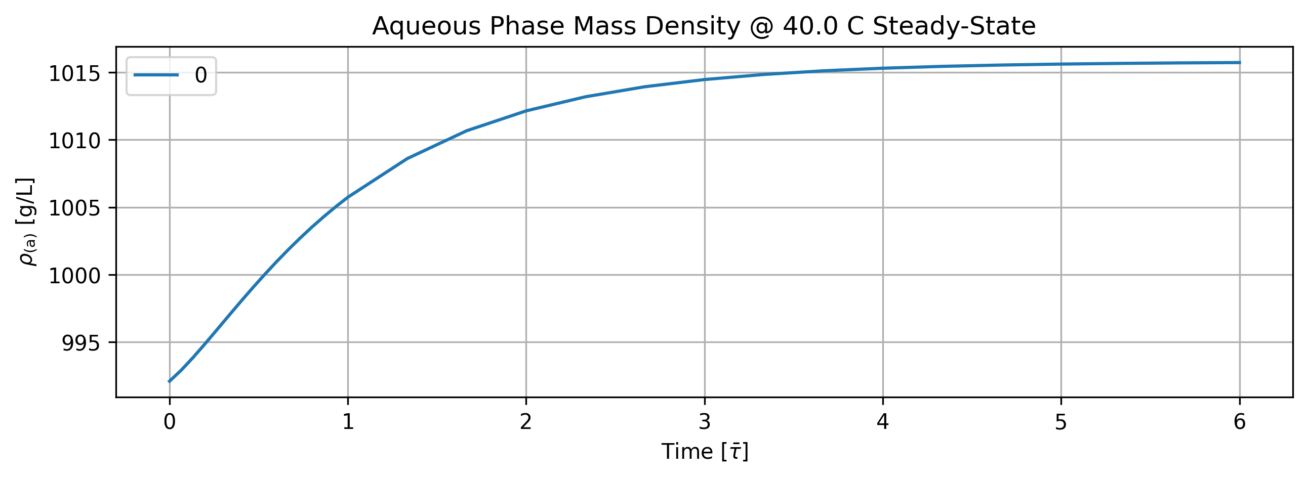
Figure 17: Aqueous phase mass density history at Steady-State.
tbl_count += 1
print(f'Table {tbl_count}: Aqueous phase mass density history at steady-state.')
print('Time [s]  Aqueous Phase Mass Density [g/L]')
print(quant.value[::5].apply(lambda x: round(x,2)))
Table 10: Aqueous phase mass density history at steady-state.
Time [s]  Aqueous Phase Mass Density [g/L]
0.000000       992.08
17.201342      996.96
34.402683     1001.85
51.604025     1005.74
137.610734    1013.94
223.617442    1015.45
309.624151    1015.74
Name: Aqueous Phase Mass Density [g/L]; Time History in [s], dtype: float64
1.6.3. Vapor Phase Results#
'''Plot vapor phase'''
# TODO: time axis normalized by phase flow residence time.
stg.vapor_phase.plot(title='Vapor Phase Steady-State', legend='Vapor Phase', nrows=2,ncols=3, show=True, figsize=[12,6])

fig_count += 1
print(f'Figure {fig_count}: Vapor phase species history dashboard at steady-state.')
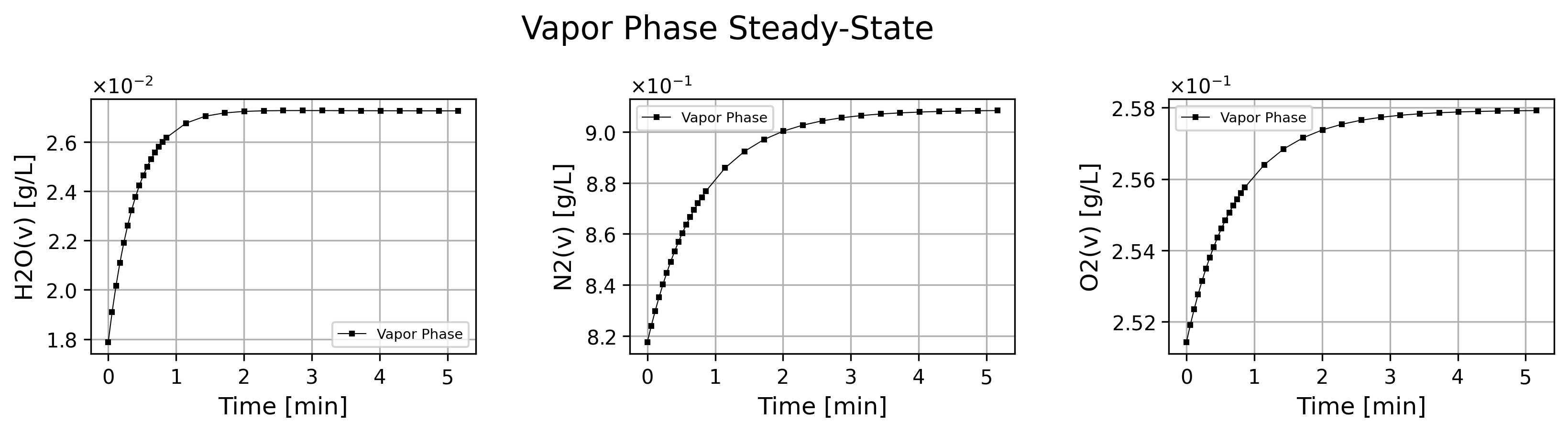
Figure 18: Vapor phase species history dashboard at steady-state.
if cortix_ai:
    issues = ('+ Title your reponse as: Overview of the Vapor Phase Data at Steady-State.\n'
              '+ Do not explain the start-up process; cover the steady-state only.'
    )
    cortix_ai.explain(phase=stg.vapor_phase, issues=issues, markdown_header_level='<h4>', markdown_display=markdown_display, save_supporting_info=db_save)
Cortix AI assistant: working on explanation...
Overview of the Vapor Phase Data at Steady-State.
Steady-state window used
Steady-state is taken as the time span t ≥ 137.611 s (rows starting at 137.611 s through 309.624 s).
Numerical summary (steady-state statistics)
H₂O(v): mean = 0.0272740 g/L; standard deviation ≈ 4.51×10⁻⁶ g/L; min = 0.0272684 g/L; max = 0.0272808 g/L; range = 1.24×10⁻⁵ g/L; coefficient of variation ≈ 0.0165%.
N₂(v): mean = 0.906763 g/L; standard deviation ≈ 1.85×10⁻³ g/L; min = 0.902695 g/L; max = 0.908398 g/L; range = 5.703×10⁻³ g/L; coefficient of variation ≈ 0.204%.
O₂(v): mean = 0.257811 g/L; standard deviation ≈ 1.24×10⁻⁴ g/L; min = 0.257538 g/L; max = 0.257921 g/L; range = 3.83×10⁻⁴ g/L; coefficient of variation ≈ 0.0482%.
Steady-state composition (mass fractions)
Total vapor concentration (steady mean sum) ≈ 1.191849 g/L.
Mass fractions: H₂O(v) ≈ 2.29% ; N₂(v) ≈ 76.13% ; O₂(v) ≈ 21.58%.
Trend and stability over the steady window
Time span used: 172.013 s (from 137.611 s to 309.624 s).
Linear changes over that window (end − start, divided by time span):
N₂(v) increased by 0.005703 g/L → slope ≈ +3.32×10⁻⁵ g·L⁻¹·s⁻¹.
O₂(v) increased by 3.83×10⁻⁴ g/L → slope ≈ +2.23×10⁻⁶ g·L⁻¹·s⁻¹.
H₂O(v) decreased by 2.7×10⁻⁶ g/L → slope ≈ −1.57×10⁻⁸ g·L⁻¹·s⁻¹.
Interpretation: all three species show very small absolute drifts and low coefficients of variation (all ≪ 1%), indicating the vapor-phase concentrations are effectively steady within the chosen window; N₂ shows the largest absolute variability and drift, O₂ shows very small variability, and H₂O is essentially constant at the 10⁻⁵ g/L level.
AI Parameters:
+ LLM model (OpenAI) = gpt-5-mini
+ LLM cleverness     = 1.0
+ Total # of tokens  = 8755
'''Vapor phase mass density'''
import matplotlib.pyplot as plt

quant = stg.mass_density_history('vapor')

quant.plot(title='Vapor Phase Mass Density @ %2.1f C Steady-State'%unit.convert_temperature(stg_temperature,
           'K','C'), x_scaling=1/stg.flow_residence_time_avg, x_label=r'Time [$\bar{\tau}$]', y_label=quant.latex_name+
           ' ['+quant.unit+']', show=True, figsize=[10,3], error_data=False)

fig_count += 1
print(f'Figure {fig_count}: Vapor phase mass density history at steady-state.')
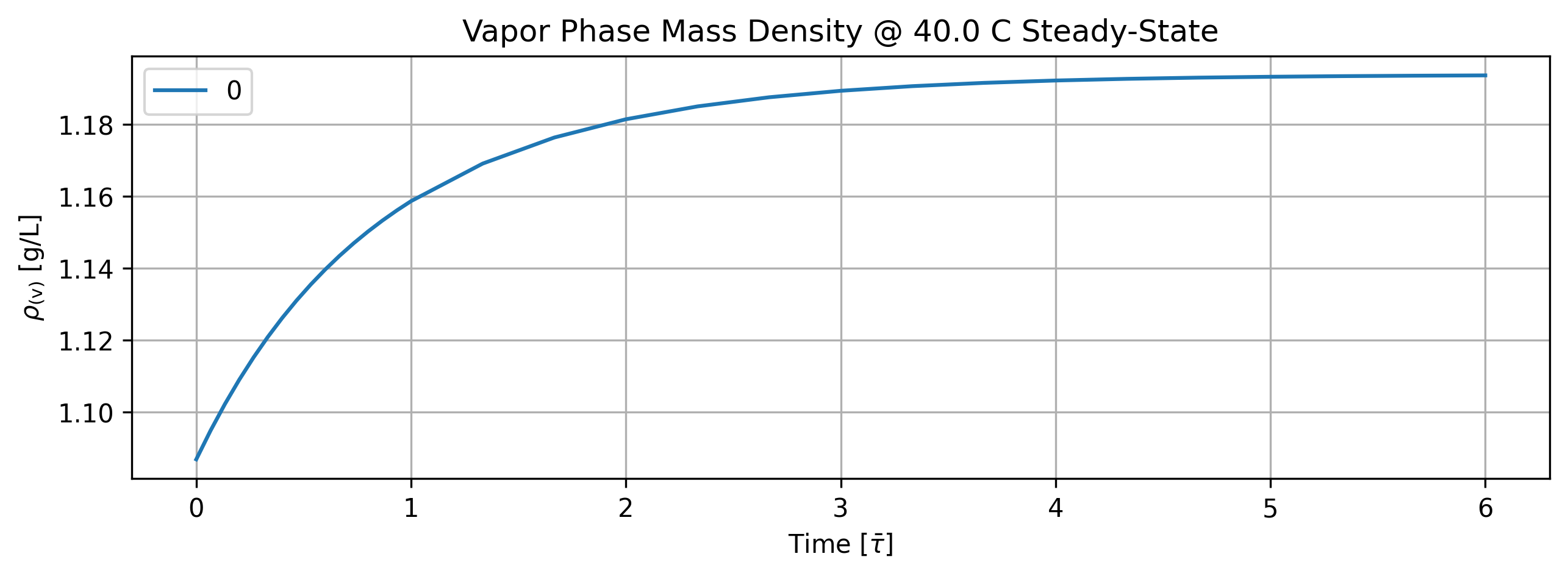
Figure 19: Vapor phase mass density history at steady-state.
tbl_count += 1
print(f'Table {tbl_count}: Vapor phase mass density history at steady-state.')
print('Time [s]  Vapor Phase Mass Density [g/L]')
print(quant.value[::5].apply(lambda x: round(x,2)))
Table 11: Vapor phase mass density history at steady-state.
Time [s]  Vapor Phase Mass Density [g/L]
0.000000      1.09
17.201342     1.12
34.402683     1.14
51.604025     1.16
137.610734    1.19
223.617442    1.19
309.624151    1.19
Name: Vapor Phase Mass Density [g/L]; Time History in [s], dtype: float64
1.6.3.1. Relative Humidity#
'''Compute relative humidity in the vapor phase'''
import matplotlib.pyplot as plt
from solvex import air_relative_humidity
from copy import deepcopy

h2o_vap_pd_series = deepcopy(stg.vapor_phase.df['H2O(v)'])
for idx, rho_h2o in enumerate(h2o_vap_pd_series):
    h2o_vap_pd_series.iloc[idx] = air_relative_humidity(stg_temperature, rho_h2o)
rh_pd_series = h2o_vap_pd_series
time_unit = stg.vapor_phase.time_unit
rh_pd_series.name = f'Relative Humidity History [{time_unit}]'

quant = Quantity(name=rh_pd_series.name, latex_name='RH', unit='%', info=f'Relative Humidity History (Vapor Phase) [{time_unit}]')
quant.value = h2o_vap_pd_series
quant.plot(title='Stage Rel. Humidity @ %2.1f C Steady-State'%unit.convert_temperature(stg_temperature, 'K','C'),
           x_scaling=1/stg.flow_residence_time_avg, x_label=r'Time [$\bar{\tau}$]', y_label=quant.latex_name+' ['+quant.unit+']', show=True,
           figsize=[10,3])

fig_count += 1
print(f'Figure {fig_count}: Stage relative humidity history at steady-state.')
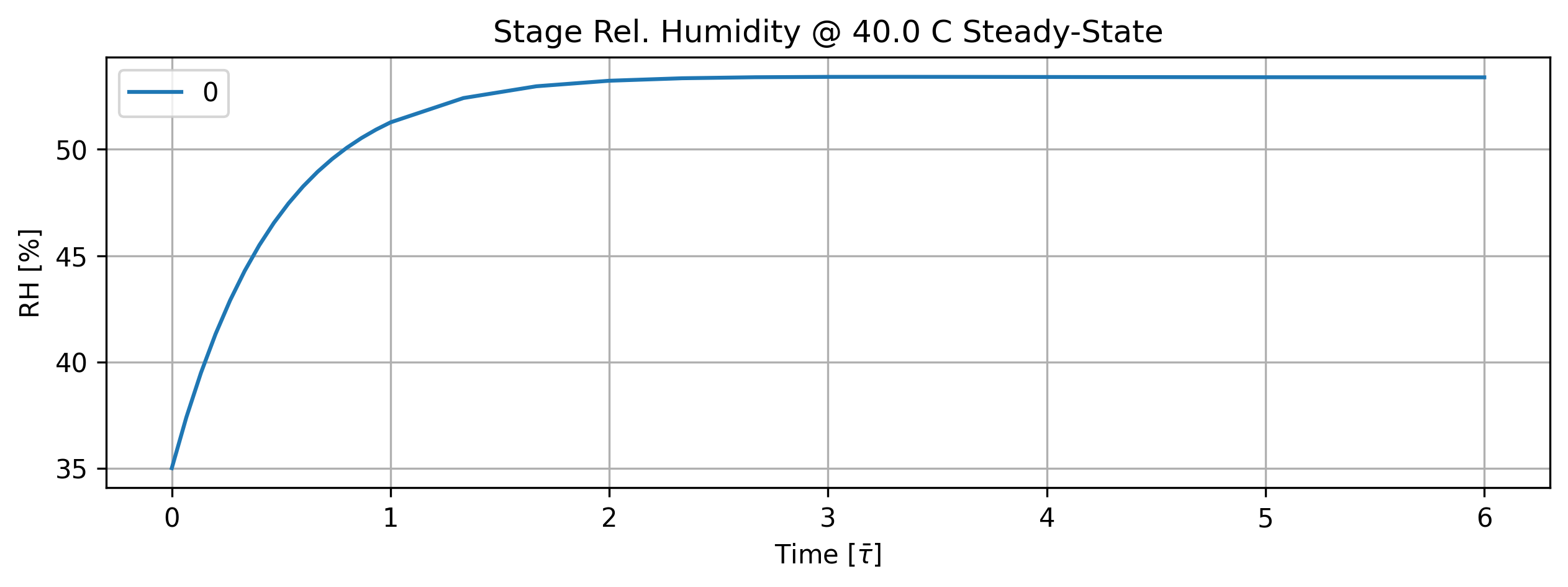
Figure 20: Stage relative humidity history at steady-state.
tbl_count += 1
print(f'Table {tbl_count}: Stage relative humidity history at steady-state.')
print('Time [s]  Rel. Humidity [%]')
print(quant.value.loc[n_startup::5].apply(lambda x: round(x,2)))
Table 12: Stage relative humidity history at steady-state.
Time [s]  Rel. Humidity [%]
17.201342     44.28
34.402683     48.95
51.604025     51.27
137.610734    53.40
223.617442    53.40
309.624151    53.39
Name: Relative Humidity History [s], dtype: float64
if cortix_ai:
    issues = ('+ Title your reponse as: Overview of the Relative Humidity Data at Steady-State.\n'
              '+ Do not explain the start-up process; cover the steady-state only.'
    )
    cortix_ai.explain(quant=quant, issues=issues, markdown_header_level='<h5>', markdown_display=markdown_display, print_prompt=False, save_supporting_info=db_save)
Cortix AI assistant: working on explanation...
Overview of the Relative Humidity Data at Steady-State
Steady-state window and sampling:
Time interval: 103.208 s to 309.624 s (duration 206.416 s).
Number of steady-state samples: 5 (indices 6–10).
Sampling interval: 51.604 s between successive steady-state time points.
Values (dependent quantity: Relative Humidity History [s], unit: %):
Observed RH values in the window: 53.2307%, 53.4125%, 53.4076%, 53.3963%, 53.3908%.
Summary statistics (steady-state subset):
Mean RH: 53.3676% (rounded to 4 decimal places).
Population standard deviation: ≈ 0.0689% (sample std ≈ 0.0770%).
Min / Max: 53.2307% / 53.4125% → range = 0.1818%.
Trend over the steady-state interval:
Linear trend (least-squares slope) ≈ +5.89 × 10⁻⁴ % per second.
Equivalent changes: ≈ +0.0353% per minute, ≈ +0.589% per 1,000 s.
Interpretation: the RH is effectively constant within ±0.1% over the interval; the positive slope is very small compared with the mean.
Concise interpretation:
Over the stated steady-state window the relative humidity is stable around 53.37% with very low variability (std ≈ 0.07% and range ≈ 0.18%) and only a negligible upward trend.
AI Parameters:
+ LLM model (OpenAI) = gpt-5-mini
+ LLM cleverness     = 1.0
+ Total # of tokens  = 5261
1.6.4. Overall Stage Efficiency#
'''Stage overall efficiency'''

quant = stg.efficiency_history(mean=True)
quant.plot(title='Stage Efficiency @ %2.1f C Steady-State'%unit.convert_temperature(stg_temperature,
           'K','C'), x_scaling=1/stg.flow_residence_time_avg, x_label=r'Time [$\bar{\tau}$]', y_label=quant.latex_name+
           ' ['+quant.unit+']', show=True, figsize=[10,3], error_data=True)

fig_count += 1
print(f'Figure {fig_count}: Stage efficiency history steady-state.')
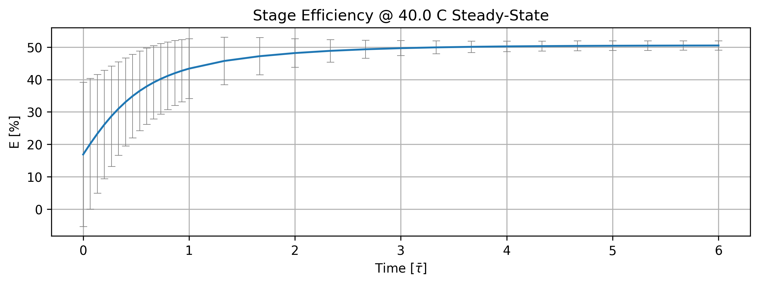
Figure 21: Stage efficiency history steady-state.
tbl_count += 1
print(f'Table {tbl_count}: Stage efficiency history at steady-state.')
print('Time [s]  (Stage. Eff., +-std) [%]')
time_name = ''
import pandas as pd
df = (quant.value.apply(pd.Series).mul(1)
       .rename(index=lambda i: round(i/unit.min,2))
       .set_axis(['',''], axis=1).rename_axis(time_name)
       .round(3))
print(df.to_string(max_rows=20, min_rows=20))
Table 13: Stage efficiency history at steady-state.
Time [s]  (Stage. Eff., +-std) [%]


0.00  16.875  22.212
0.06  20.172  20.127
0.11  23.258  18.305
0.17  26.106  16.757
0.23  28.693  15.478
0.29  31.001  14.440
0.34  33.063  13.593
0.40  34.884  12.895
0.46  36.484  12.303
0.52  37.888  11.783
...      ...     ...
2.58  49.669   2.304
2.87  49.915   1.982
3.15  50.092   1.776
3.44  50.218   1.646
3.73  50.309   1.565
4.01  50.374   1.515
4.30  50.420   1.484
4.59  50.454   1.464
4.87  50.478   1.451
5.16  50.495   1.442
if cortix_ai:
    issues = ('+ Title your reponse as: Overview of the Stage Efficiency Data at Steady-State.\n'
              '+ Do not explain the start-up process; cover the steady-state only.'
    )
    cortix_ai.explain(quant=quant, issues=issues, markdown_header_level='<h4>', markdown_display=markdown_display, save_supporting_info=db_save)
Cortix AI assistant: working on explanation...
Overview of the Stage Efficiency Data at Steady-State
Steady-state definition and span.
Steady-state is taken as the interval t ≥ 103.208 s (rows 6–10), covering 103.208 s to 309.624 s with regular sampling steps of ≈ 51.604 s.
Time [s] column (sampling).
Times in the steady window are: 103.208, 154.812, 206.416, 258.020, 309.624 s; spacing is consistent at ≈ 51.604 s.
Mean efficiency column (reported mean [%]).
Reported means in the steady window: 48.1704%, 49.6695%, 50.2183%, 50.4204%, 50.4947%.
Average (mean of those five values) = 49.79% (49.7947%).
Variability of the reported mean across the steady window: sample standard deviation ≈ 0.96% (population std ≈ 0.86%), indicating the mean is approximately stable with only ~0.9–1.0 percentage point scatter.
Final reported mean (last time point) = 50.49%.
Reported uncertainty column (reported ± std [%]).
Reported standard deviations in the steady window: 4.44318%, 2.30373%, 1.64574%, 1.48376%, 1.44219%.
Mean reported uncertainty across the steady window = 2.26% (2.2637%).
Uncertainty decreases through the steady window from 4.44% to 1.44% (a reduction of ≈ 67.5% between first and last steady samples).
Relative uncertainty (coefficient of variation = reported std ÷ mean) falls from ≈ 9.2% at 103.208 s to ≈ 2.9% at 309.624 s (using the corresponding means).
Concise quantitative summary.
Steady-window average efficiency = 49.79% ± 0.96% (sample std across times).
Typical reported measurement uncertainty = 2.26% (mean of reported std values); last reported point = 50.49% ± 1.44% (reported std).
Conclusion: over the chosen steady interval the stage efficiency is centered near 50% with small temporal scatter (~1% absolute) and decreasing reported uncertainty toward the final measurement.
AI Parameters:
+ LLM model (OpenAI) = gpt-5-mini
+ LLM cleverness     = 1.0
+ Total # of tokens  = 4923
'''Individual reaction efficiency'''

quant = stg.efficiency_history()
quant.plot(title='Reaction Efficiency @ %2.1f C Steady-State'%unit.convert_temperature(stg_temperature,
           'K','C'), x_scaling=1/stg.flow_residence_time_avg, x_label=r'Time [$\bar{\tau}$]', y_label=quant.latex_name+
           ' ['+quant.unit+']', legend=stg.rxn_mech.reactions, show=True, figsize=[10,3])

fig_count += 1
print(f'Figure {fig_count}: Reaction efficiency history at steady-state.')
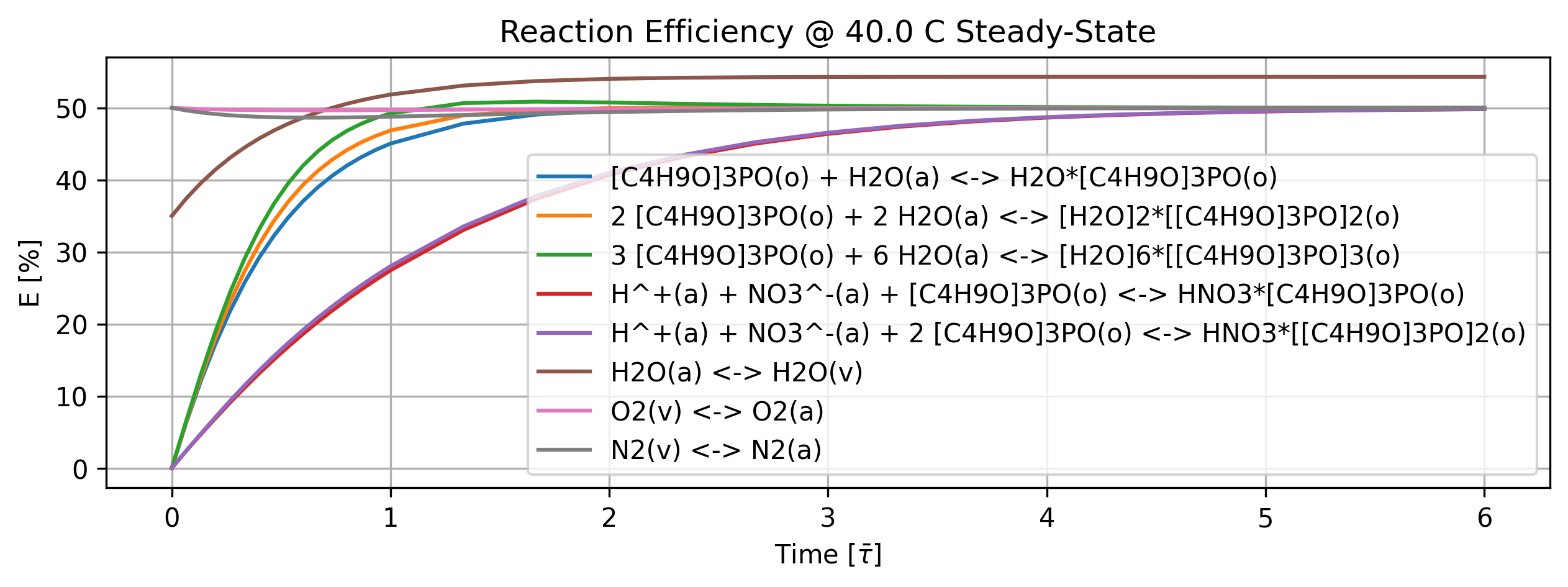
Figure 22: Reaction efficiency history at steady-state.
'''Individual reaction efficiency'''
quant = stg.efficiency_history()
tbl_count += 1
print(f'Table {tbl_count}: Reaction efficiency history at steady-state.')
print('Time [min]    Rxn Eff. [%]')

col_names = [f'r{i}' for i in range(len(stg.rxn_mech.reactions))]
time_name = ''
df = (quant.value.apply(pd.Series).mul(1)
       .rename(index=lambda i: round(i/unit.min,2))
       .set_axis(col_names, axis=1).rename_axis(time_name)
       .round(3))
print(df.to_string(max_rows=20, min_rows=20))
Table 14: Reaction efficiency history at steady-state.
Time [min]    Rxn Eff. [%]
          r0      r1      r2      r3      r4      r5      r6      r7

0.00   0.000   0.000   0.000   0.000   0.000  35.002  50.000  50.000
0.06   6.372   6.506   6.645   2.416   2.443  37.442  49.910  49.642
0.11  12.132  12.583  13.058   4.712   4.802  39.578  49.839  49.359
0.17  17.274  18.119  19.025   6.943   7.114  41.447  49.783  49.140
0.23  21.816  23.063  24.417   9.099   9.356  43.082  49.741  48.972
0.29  25.784  27.351  29.114  11.174  11.512  44.513  49.710  48.847
0.34  29.247  31.098  33.208  13.165  13.576  45.763  49.688  48.758
0.40  32.244  34.304  36.682  15.069  15.541  46.857  49.674  48.698
0.46  34.829  37.023  39.587  16.889  17.409  47.813  49.665  48.661
0.52  37.050  39.311  41.987  18.625  19.180  48.648  49.661  48.644
...      ...     ...     ...     ...     ...     ...     ...     ...
2.58  50.036  50.047  50.303  46.398  46.563  54.289  49.946  49.774
2.87  50.045  50.038  50.219  47.397  47.525  54.303  49.961  49.836
3.15  50.043  50.029  50.157  48.123  48.221  54.308  49.972  49.882
3.44  50.036  50.021  50.113  48.649  48.723  54.309  49.980  49.915
3.73  50.028  50.016  50.081  49.028  49.084  54.309  49.986  49.939
4.01  50.022  50.011  50.058  49.302  49.344  54.308  49.990  49.956
4.30  50.016  50.008  50.042  49.499  49.530  54.307  49.993  49.969
4.59  50.012  50.006  50.030  49.641  49.663  54.306  49.995  49.978
4.87  50.009  50.004  50.022  49.742  49.759  54.306  49.996  49.984
5.16  50.006  50.003  50.015  49.815  49.827  54.305  49.997  49.988
if cortix_ai:
    issues = ('+ Title your reponse as: Overview of Individual Reaction Efficiency at Steady-State'
             '+ Do not explain the start-up process; cover the steady-state only.'
    )
    cortix_ai.explain(quant=quant, issues=issues, markdown_header_level='<h4>', markdown_display=markdown_display, save_supporting_info=db_save)
Cortix AI assistant: working on explanation...
Overview of Individual Reaction Efficiency at Steady-State+
Steady-state window used for this analysis: times t ≥ 103.208 s (rows 6–10). Below are per-reaction steady-state statistics (mean, min, max, range) and a concise stability note.
[C₄H₉O]₃PO(o) + H₂O(a) <-> H₂O·[C₄H₉O]₃PO(o)
Mean = 49.946% ; Min = 49.637% ; Max = 50.036% ; Range = 0.399%
Very stable around 50% with negligible fluctuation.
2 [C₄H₉O]₃PO(o) + 2 H₂O(a) <-> [H₂O]₂·[[C₄H₉O]₃PO]₂(o)
Mean = 50.008% ; Min = 49.961% ; Max = 50.047% ; Range = 0.086%
Highly stable, essentially constant at 50%.
3 [C₄H₉O]₃PO(o) + 6 H₂O(a) <-> [H₂O]₆·[[C₄H₉O]₃PO]₃(o)
Mean = 50.243% ; Min = 50.016% ; Max = 50.744% ; Range = 0.728%
Centered slightly above 50% with small remaining variability.
H⁺(a) + NO₃⁻(a) + [C₄H₉O]₃PO(o) <-> HNO₃·[C₄H₉O]₃PO(o)
Mean = 47.010% ; Min = 40.691% ; Max = 49.815% ; Range = 9.124%
Largest spread in the steady window; efficiency increased substantially across the window and approaches ~49–50% by the final times.
H⁺(a) + NO₃⁻(a) + 2 [C₄H₉O]₃PO(o) <-> HNO₃·[[C₄H₉O]₃PO]₂(o)
Mean = 47.131% ; Min = 41.014% ; Max = 49.827% ; Range = 8.813%
Similar behavior to the previous NO₃⁻-associated reaction: notable rise through the steady window, nearing 50% at the end.
H₂O(a) <-> H₂O(v)
Mean = 54.249% ; Min = 54.033% ; Max = 54.309% ; Range = 0.276%
Highest efficiency among all reactions and very stable (≈54.3%).
O₂(v) <-> O₂(a)
Mean = 49.955% ; Min = 49.861% ; Max = 49.997% ; Range = 0.137%
Stable and tightly clustered around 50%.
N₂(v) <-> N₂(a)
Mean = 49.814% ; Min = 49.423% ; Max = 49.988% ; Range = 0.565%
Close to 50% with small remaining upward drift across the window.
Summary observation
Most reactions occupy ≈50% efficiency at steady-state with very small variability (ranges ≲0.8%) except the two NO₃⁻-associated uptake reactions (the HNO₃ adducts), which show larger changes across the chosen steady-state interval (ranges ≈8.8–9.1%) and approach ~49–50% by the final time points. H₂O(a) <-> H₂O(v) is distinctively higher (~54.3%).
AI Parameters:
+ LLM model (OpenAI) = gpt-5-mini
+ LLM cleverness     = 1.0
+ Total # of tokens  = 6729
1.6.5. Reaction Rate Density#
This quantity only makes sense per volume of the mixture.
'''Reaction rate density'''
import matplotlib.pyplot as plt

quant = stg.r_vec_history()# mole/m^3-s

quant.plot(title='Reaction Rate Density @ %2.1f C Steady-State'%unit.convert_temperature(stg_temperature,
           'K','C'), x_scaling=1/stg.flow_residence_time_avg, x_label=r'Time [$\bar{\tau}$]', y_label=quant.latex_name+
           ' ['+quant.unit+']', legend=stg.rxn_mech.reactions, show=True, figsize=[10,3], error_data=False)

fig_count += 1
print(f'Figure {fig_count}: Reaction rate density history at steady-state.')
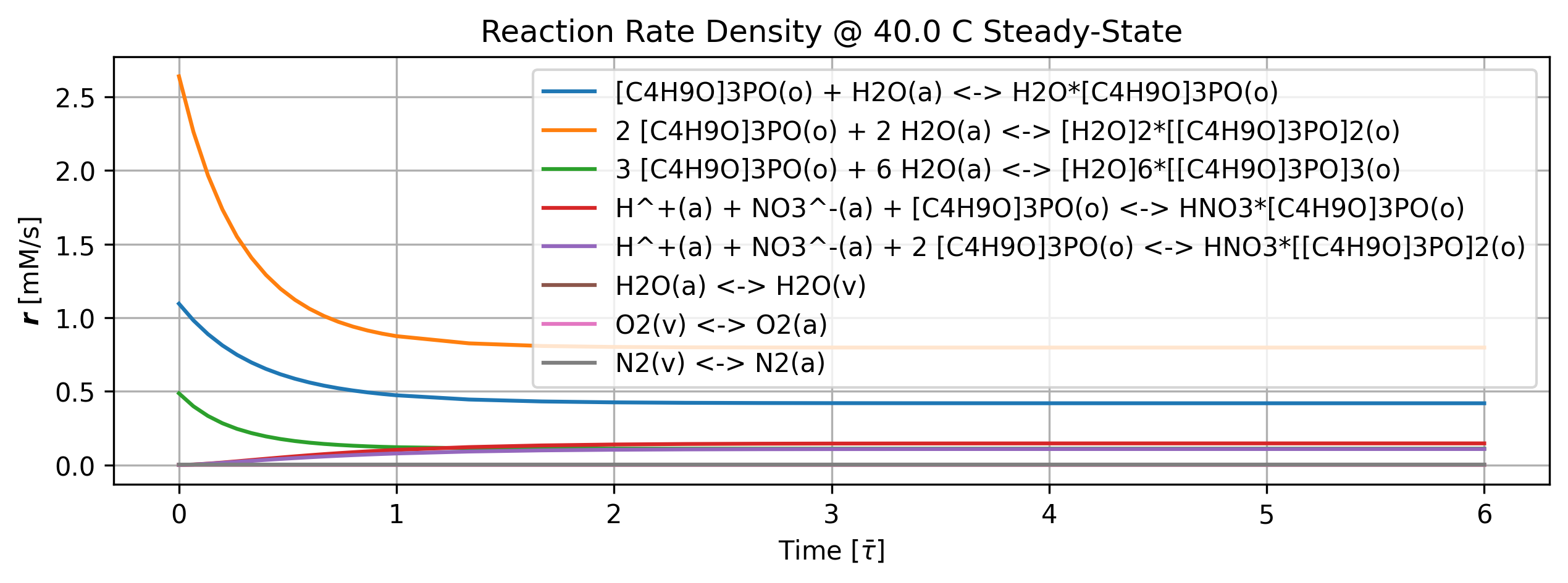
Figure 23: Reaction rate density history at steady-state.
tbl_count += 1
print(f'Table {tbl_count}: Reaction rate density history at steady-state.')
print('Time [min]      r [mM/s]')
import pandas as pd
col_names = [f'r{i}' for i in range(len(stg.rxn_mech.reactions))]
time_name = 't [min]'
df = (quant.value.apply(pd.Series).mul(1)
       .rename(index=lambda i: round(i/unit.min,2))
       .set_axis(col_names, axis=1).rename_axis(time_name)
       .round(4))
print(df.iloc[n_startup:].to_string(max_rows=20, min_rows=20))
Table 15: Reaction rate density history at steady-state.
Time [min]      r [mM/s]
             r0      r1      r2      r3      r4      r5      r6      r7
t [min]
1.15     0.4446  0.8261  0.1136  0.1214  0.0914  0.0014  0.0014  0.0027
1.43     0.4315  0.8083  0.1115  0.1326  0.0991  0.0014  0.0014  0.0027
1.72     0.4253  0.8017  0.1109  0.1390  0.1035  0.0013  0.0014  0.0027
2.01     0.4222  0.7992  0.1107  0.1425  0.1058  0.0013  0.0014  0.0027
2.29     0.4207  0.7982  0.1106  0.1444  0.1070  0.0013  0.0014  0.0027
2.58     0.4200  0.7978  0.1106  0.1454  0.1077  0.0013  0.0014  0.0027
2.87     0.4196  0.7976  0.1106  0.1459  0.1080  0.0013  0.0014  0.0027
3.15     0.4194  0.7976  0.1106  0.1462  0.1081  0.0013  0.0014  0.0027
3.44     0.4192  0.7976  0.1106  0.1463  0.1082  0.0013  0.0014  0.0027
3.73     0.4192  0.7975  0.1106  0.1464  0.1083  0.0013  0.0014  0.0027
4.01     0.4192  0.7975  0.1106  0.1465  0.1083  0.0013  0.0014  0.0027
4.30     0.4191  0.7975  0.1106  0.1465  0.1083  0.0013  0.0014  0.0027
4.59     0.4191  0.7975  0.1106  0.1465  0.1083  0.0013  0.0014  0.0027
4.87     0.4191  0.7975  0.1106  0.1465  0.1083  0.0013  0.0014  0.0027
5.16     0.4191  0.7975  0.1106  0.1465  0.1083  0.0013  0.0014  0.0027
if cortix_ai:
    issues = ('+ Title your reponse as: Overview of Reaction Rates Density at Steady-State.\n'
              '+ Do not explain the start-up process; cover the steady-state only.'
)
    cortix_ai.explain(quant=quant, issues=issues, markdown_header_level='<h4>', markdown_display=markdown_display, print_prompt=False, save_supporting_info=db_save)
Cortix AI assistant: working on explanation...
Overview of Reaction Rates Density at Steady-State
Steady-state snapshot (final time point)
Values reported are the reaction-rate densities [mM/s] taken at the final time (309.624 s). The eight columns correspond to the ordered reactions listed below (index → reaction).
Reaction index mapping (converted to required chemical formatting; reversible reactions use “<=>”):
0 → [C₄H₉O]₃PO(o) + H₂O(a) <=> H₂O·[C₄H₉O]₃PO(o)
1 → 2 [C₄H₉O]₃PO(o) + 2 H₂O(a) <=> [H₂O]₂·[[C₄H₉O]₃PO]₂(o)
2 → 3 [C₄H₉O]₃PO(o) + 6 H₂O(a) <=> [H₂O]₆·[[C₄H₉O]₃PO]₃(o)
3 → H⁺(a) + NO₃⁻(a) + [C₄H₉O]₃PO(o) <=> HNO₃·[C₄H₉O]₃PO(o)
4 → H⁺(a) + NO₃⁻(a) + 2 [C₄H₉O]₃PO(o) <=> HNO₃·[[C₄H₉O]₃PO]₂(o)
5 → H₂O(a) <=> H₂O(v)
6 → O₂(v) <=> O₂(a)
7 → N₂(v) <=> N₂(a)
Numeric steady-state rates and relative contributions
Total summed reaction-rate density (final time): 1.587518 mM/s
Per-reaction steady-state values (mM/s) and fraction of the total:
Reaction 0: 0.419134 mM/s (26.4% of total)
Reaction 1: 0.797538 mM/s (50.2% of total)
Reaction 2: 0.110605 mM/s (7.0% of total)
Reaction 3: 0.146490 mM/s (9.2% of total)
Reaction 4: 0.108296 mM/s (6.8% of total)
Reaction 5: 0.00133096 mM/s (0.08% of total)
Reaction 6: 0.00142770 mM/s (0.09% of total)
Reaction 7: 0.00269596 mM/s (0.17% of total)
Key steady-state observations
Liquid-phase complexation/solvation reactions dominate the steady-state flux: reactions 0–4 together account for ≈99.9% of the total reaction-rate density, with reaction 1 (the 2:2 complex formation) being the single largest contributor (~50%).
Gas–liquid transfer reactions (indices 5–7: H₂O, O₂, N₂ exchanges) are negligible at steady-state (each <0.2% of total), so their rates are minor compared with the liquid-phase chemistry.
Stability across final time points: the reported final values are essentially steady — values at the last three sampled times (206.416 s, 258.02 s, 309.624 s) show only very small relative changes (all changes ≪ 0.2%, most ≪ 0.1%), confirming a steady-state regime for the rates listed above.
AI Parameters:
+ LLM model (OpenAI) = gpt-5-mini
+ LLM cleverness     = 1.0
+ Total # of tokens  = 6333
1.6.6. Species Generation Rate Density#
This quantity is on the basis of mixing volume so all species generation values can be compared.
'''Species generation rate density'''
import matplotlib.pyplot as plt

quant = stg.g_vec_history() # mole/m^3-s

quant.plot(title='Species Generation Rate Density @ %2.1f C Steady-State'%unit.convert_temperature(stg_temperature,
           'K','C'), x_scaling=1/stg.flow_residence_time_avg, x_label=r'Time [$\bar{\tau}$]', y_label=quant.latex_name+
           ' ['+quant.unit+']', legend=stg.rxn_mech.species_names, show=True, figsize=[10,3], error_data=False)

fig_count += 1
print(f'Figure {fig_count}: Species generation rate density history at steady-state.')
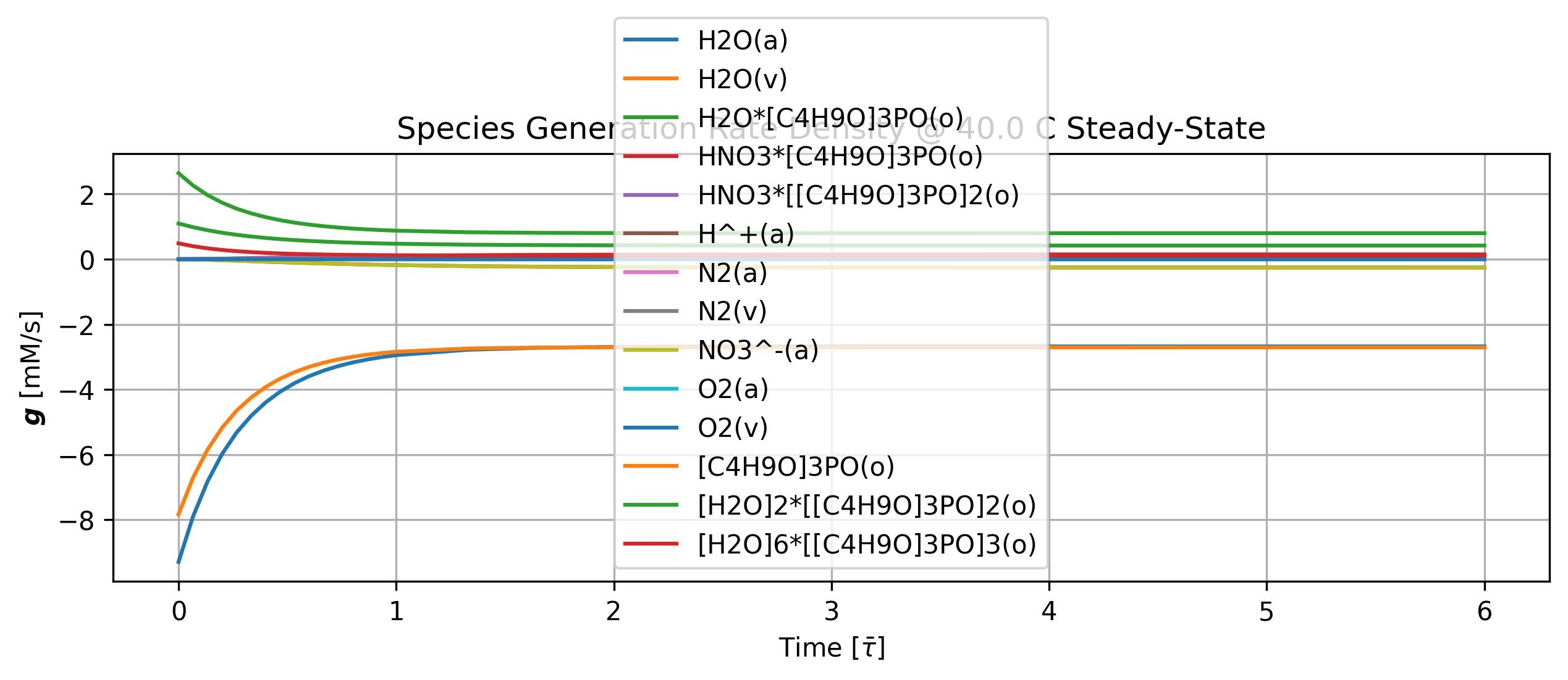
Figure 24: Species generation rate density history at steady-state.
tbl_count += 1
print(f'Table {tbl_count}: Species generation rate density history at steady-state.')
print('Time [min]        g [mM/s]')
import pandas as pd
col_names = [f'a{i}' for i in range(len(stg.rxn_mech.species_names))]
time_name = 't [min]'
df = (quant.value.apply(pd.Series).mul(1)
       .rename(index=lambda i: round(i/unit.min,2))
       .set_axis(col_names, axis=1).rename_axis(time_name)
       .round(4))
print(df.iloc[n_startup:].to_string(max_rows=20, min_rows=20))
Table 16: Species generation rate density history at steady-state.
Time [min]        g [mM/s]
             a0      a1      a2      a3      a4      a5      a6      a7      a8      a9     a10     a11     a12     a13
t [min]
1.15    -2.7799  0.0014  0.4446  0.1214  0.0914 -0.2127  0.0027 -0.0027 -0.2127  0.0014 -0.0014 -2.7418  0.8261  0.1136
1.43    -2.7184  0.0014  0.4315  0.1326  0.0991 -0.2317  0.0027 -0.0027 -0.2317  0.0014 -0.0014 -2.7134  0.8083  0.1115
1.72    -2.6952  0.0013  0.4253  0.1390  0.1035 -0.2425  0.0027 -0.0027 -0.2425  0.0014 -0.0014 -2.7072  0.8017  0.1109
2.01    -2.6860  0.0013  0.4222  0.1425  0.1058 -0.2483  0.0027 -0.0027 -0.2483  0.0014 -0.0014 -2.7068  0.7992  0.1107
2.29    -2.6822  0.0013  0.4207  0.1444  0.1070 -0.2514  0.0027 -0.0027 -0.2514  0.0014 -0.0014 -2.7075  0.7982  0.1106
2.58    -2.6806  0.0013  0.4200  0.1454  0.1077 -0.2531  0.0027 -0.0027 -0.2531  0.0014 -0.0014 -2.7081  0.7978  0.1106
2.87    -2.6798  0.0013  0.4196  0.1459  0.1080 -0.2539  0.0027 -0.0027 -0.2539  0.0014 -0.0014 -2.7086  0.7976  0.1106
3.15    -2.6795  0.0013  0.4194  0.1462  0.1081 -0.2543  0.0027 -0.0027 -0.2543  0.0014 -0.0014 -2.7088  0.7976  0.1106
3.44    -2.6793  0.0013  0.4192  0.1463  0.1082 -0.2546  0.0027 -0.0027 -0.2546  0.0014 -0.0014 -2.7090  0.7976  0.1106
3.73    -2.6792  0.0013  0.4192  0.1464  0.1083 -0.2547  0.0027 -0.0027 -0.2547  0.0014 -0.0014 -2.7090  0.7975  0.1106
4.01    -2.6792  0.0013  0.4192  0.1465  0.1083 -0.2547  0.0027 -0.0027 -0.2547  0.0014 -0.0014 -2.7091  0.7975  0.1106
4.30    -2.6792  0.0013  0.4191  0.1465  0.1083 -0.2548  0.0027 -0.0027 -0.2548  0.0014 -0.0014 -2.7091  0.7975  0.1106
4.59    -2.6792  0.0013  0.4191  0.1465  0.1083 -0.2548  0.0027 -0.0027 -0.2548  0.0014 -0.0014 -2.7091  0.7975  0.1106
4.87    -2.6792  0.0013  0.4191  0.1465  0.1083 -0.2548  0.0027 -0.0027 -0.2548  0.0014 -0.0014 -2.7091  0.7975  0.1106
5.16    -2.6792  0.0013  0.4191  0.1465  0.1083 -0.2548  0.0027 -0.0027 -0.2548  0.0014 -0.0014 -2.7091  0.7975  0.1106
'''Produced species generation rate density'''
import matplotlib.pyplot as plt

ids, quant_produced = stg.g_vec_history(produced=True) # mole/m^3-s

quant_produced.plot(title='Produced Species Generation Rate Density @ %2.1f C Steady-State'%unit.convert_temperature(stg_temperature,
           'K','C'), x_scaling=1/stg.flow_residence_time_avg, x_label=r'Time [$\bar{\tau}$]', y_label=quant.latex_name+
           ' ['+quant_produced.unit+']', legend=list(np.array(stg.rxn_mech.species_names)[ids]), show=True, figsize=[10,3], error_data=False)

fig_count += 1
print(f'Figure {fig_count}: Produced species generation rate density history at steady-state.')
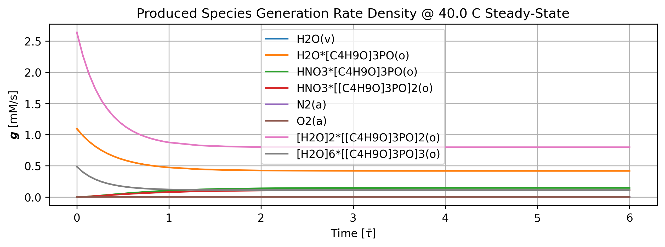
Figure 25: Produced species generation rate density history at steady-state.
if cortix_ai:
    issues = ('+ Title your reponse as: Overview of Species Generation Rates Density at Steady-State.\n'
              '+ Do not explain the start-up process; cover the steady-state only.\n'
              '+ Identify the groups of produced species and consumed species.'
)
    cortix_ai.explain(quant=quant, issues=issues, markdown_header_level='<h4>', markdown_display=markdown_display, print_prompt=False, save_supporting_info=db_save)
Cortix AI assistant: working on explanation...
Overview of Species Generation Rates Density at Steady-State.
Steady-state taken from times 103.208 s through 309.624 s (rows 6–10); values are effectively constant over that interval. Reported generation rates are in mM/s and represent mean behaviour in the steady regime.
Summary of steady-state tendencies (mean generation rates, mM/s)
H₂O(a): -2.683 mM/s (consumed)
H₂O(v): 0.001333 mM/s (produced)
H₂O·[C₄H₉O]₃PO(o): 0.4206 mM/s (produced)
HNO₃·[C₄H₉O]₃PO(o): 0.1447 mM/s (produced)
HNO₃·[[C₄H₉O]₃PO]₂(o): 0.1072 mM/s (produced)
H⁺(a): -0.2519 mM/s (consumed)
N₂(a): 0.002695 mM/s (produced)
N₂(v): -0.002695 mM/s (consumed)
NO₃⁻(a): -0.2519 mM/s (consumed)
O₂(a): 0.0014276 mM/s (produced)
O₂(v): -0.0014276 mM/s (consumed)
[C₄H₉O]₃PO(o): -2.7085 mM/s (consumed)
[H₂O]₂·[[C₄H₉O]₃PO]₂(o): 0.7976 mM/s (produced)
[H₂O]₆·[[C₄H₉O]₃PO]₃(o): 0.11066 mM/s (produced)
Groups of produced species (net positive generation at steady-state)
Small-gas species: H₂O(v), N₂(a), O₂(a) — low positive rates (~10⁻³ mM/s)
Condensed-phase complexes and adducts: H₂O·[C₄H₉O]₃PO(o), HNO₃·[C₄H₉O]₃PO(o), HNO₃·[[C₄H₉O]₃PO]₂(o), [H₂O]₂·[[C₄H₉O]₃PO]₂(o), [H₂O]₆·[[C₄H₉O]₃PO]₃(o) — moderate to large positive rates (0.11–0.80 mM/s), with the largest being [H₂O]₂·[[C₄H₉O]₃PO]₂(o) (~0.798 mM/s)
Groups of consumed species (net negative generation at steady-state)
Bulk/parent species: [C₄H₉O]₃PO(o) and H₂O(a) — large consumption (~ -2.71 and -2.68 mM/s)
Ionic and vibrationally excited species: H⁺(a), NO₃⁻(a) (~ -0.252 mM/s each) and N₂(v), O₂(v) (small negative ~ -1–3×10⁻³ mM/s)
Key steady-state observations (concise)
The dominant consumption is of [C₄H₉O]₃PO(o) and aqueous H₂O(a); concurrently, multiple hydrated/adducted condensed species are formed, indicating net sequestration of the parent organic into hydrated complexes at steady-state.
H⁺(a) and NO₃⁻(a) have nearly equal negative rates (~ -0.252 mM/s), indicating paired removal of these ionic species at the same rate in steady-state.
Gas-phase formation (H₂O(v), N₂(a), O₂(a)) is present but at orders of magnitude lower rates than condensed-phase transformations.
AI Parameters:
+ LLM model (OpenAI) = gpt-5-mini
+ LLM cleverness     = 1.0
+ Total # of tokens  = 8111
1.6.7. Mass Balance Residual#
This is actually the total mass generation rate density (mixing volume) residual; a small number in view of total mass conservation.
'''Mass balance residuals'''
import matplotlib.pyplot as plt

quant = stg.mass_balance_residual_history()

quant.plot(title='Total Mass Generation Rate Density @ %2.1f C Steady-State'%unit.convert_temperature(stg_temperature,
           'K','C'), x_scaling=1/stg.flow_residence_time_avg, x_label=r'Time [$\bar{\tau}$]', y_label=quant.latex_name+
           ' ['+quant.unit+']', markers_only=True, legend=['Residual'], show=True, figsize=[10,3])

fig_count += 1
print(f'Figure {fig_count}: Total mass generation rate density residual history at steady-state.')
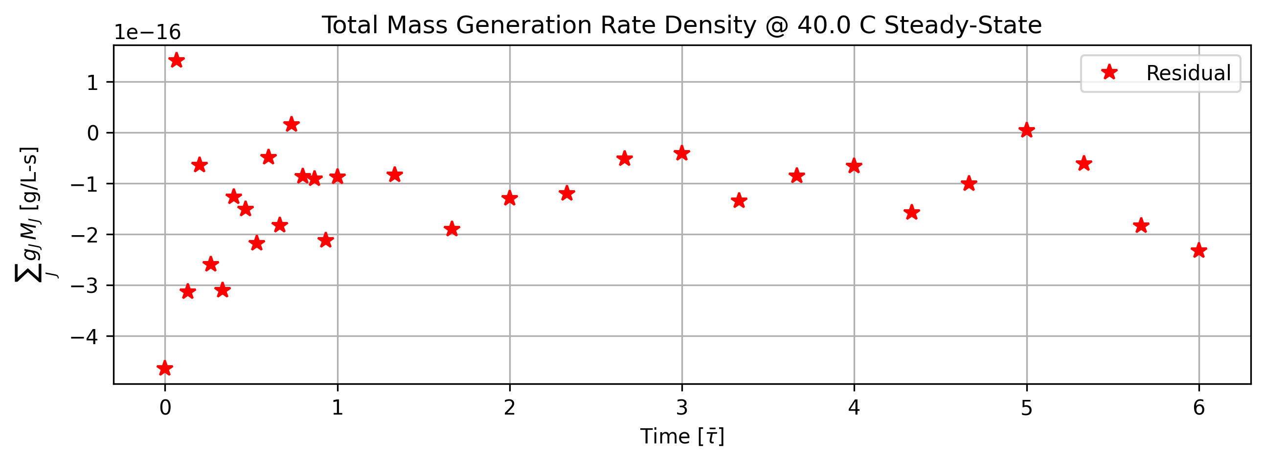
Figure 26: Total mass generation rate density residual history at steady-state.
if cortix_ai:
    issues = ('+ Title your reponse as: Total Mass Generation Rate Density Residual at Steady-State.\n'
             '+ Do not explain the start-up process; cover the steady-state only.'
    )
    cortix_ai.explain(quant=quant, issues=issues, markdown_header_level='<h4>', markdown_display=markdown_display, print_prompt=False, save_supporting_info=db_save)
Cortix AI assistant: working on explanation...
Total Mass Generation Rate Density Residual at Steady-State.
Steady-state window used: times 103.208 s → 309.624 s (last five table entries). The following quantifies the Total Mass Generation Rate Density residuals in that window.
Number of samples: 5
Time interval covered: 103.208 s, 154.812 s, 206.416 s, 258.02 s, 309.624 s
Values (g/L·s): -1.29725e-16, -4.14843e-17, -6.65294e-17, 3.93701e-18, -2.32832e-16
Mean residual: -9.33e-17 g/L·s
Median residual: -6.65e-17 g/L·s
Root-mean-square (RMS): 1.24e-16 g/L·s
Standard deviation (population): 8.12e-17 g/L·s
Maximum absolute residual: 2.32832e-16 g/L·s (at 309.624 s)
Sign / interpretation: small negative mean (bias toward sink) but all values are on the order of 10⁻¹⁶–10⁻¹⁷ g/L·s, i.e., effectively zero within numerical precision; mass balance is satisfied at steady-state to within ~1e-16 g/L·s.
AI Parameters:
+ LLM model (OpenAI) = gpt-5-mini
+ LLM cleverness     = 1.0
+ Total # of tokens  = 5201
1.7. Shut-down Simulation#
From steady-state, shutdown in three flow residence times.
end_time += 3 * stg.flow_residence_time_avg
time_step = 3 * stg.flow_residence_time_avg / 20
show_time = (True, 10*time_step)

stg.time_step = time_step
stg.initial_time = stg.end_time
stg.end_time = end_time
stg.show_time = show_time
'''Abrupt turn-off of TBP concentration in the organic phase in the inflow'''
tbp_mass_cc_org = 0.0
stg.inflow_organic_phase.set_value(tbp_org_name, tbp_mass_cc_org)
'''Run system in parallel'''
stg.monitor_mass_flowrates = False
stg.monitor_mass_conservation_residual = False
system.run()
system.close() # Shutdown Cortix
[11440] 2025-11-19 23:37:30,898 - cortix - INFO - Launching Module <solvex.stage.Stage object at 0x7f42e67c8690>
[13688] 2025-11-19 23:37:32,061 - cortix - INFO - Stg-1::run():time[m]=5.2
[13688] 2025-11-19 23:37:32,422 - cortix - INFO - Stg-1::run():time[m]=6.5
Total mass rate density (mixture volume) residual [g/L-s]= 1.19940e-18
total mass inflow rate [g/min]   = 5.118e+02
total mass outflow rate [g/min]  =  5.202e+02
	 net total mass flow rate [g/min] = 8.384e+00
[13688] 2025-11-19 23:37:32,777 - cortix - INFO - Stg-1::run():time[m]=7.7 (et[s]=0.7)
[11440] 2025-11-19 23:37:32,962 - cortix - INFO - run()::Elapsed wall clock time [s]: 1326.65
[11440] 2025-11-19 23:37:32,963 - cortix - INFO - Closed Cortix object.
_____________________________________________________________________________
                           T E R M I N A T I N G
_____________________________________________________________________________
      ...                                        s       .     (TAAG Fraktur)
   xH88"`~ .x8X                                 :8      @88>
 :8888   .f"8888Hf        u.      .u    .      .88      %8P      uL   ..
:8888>  X8L  ^""`   ...ue888b   .d88B :@8c    :888ooo    .     .@88b  @88R
X8888  X888h        888R Y888r ="8888f8888r -*8888888  .@88u  ""Y888k/"*P
88888  !88888.      888R I888>   4888>"88"    8888    888E`    Y888L
88888   %88888      888R I888>   4888> "      8888      888E      8888
88888 `> `8888>     888R I888>   4888>        8888      888E      `888N
`8888L %  ?888   ! u8888cJ888   .d888L .+    .8888Lu=   888E   .u./"888&
 `8888  `-*""   /   "*888*P"    ^"8888*"     ^%888*     888&  d888" Y888*"
   "888.      :"      "Y"          "Y"         "Y"      R888" ` "Y   Y"
     `""***~"`                                           ""
                             https://cortix.org
_____________________________________________________________________________
[11440] 2025-11-19 23:37:32,964 - cortix - INFO - close()::Elapsed wall clock time [s]: 1326.65
'''Recover stage'''
stg = system_net.modules[0]
1.7.1. Organic Phase Results#
'''Plot organic phase'''
# TODO: time axis normalized by phase flow residence time.
stg.organic_phase.plot(title='Organic Phase Shut-Down', legend='Organic Phase', nrows=2,ncols=3, show=True, figsize=[12,6])

fig_count += 1
print(f'Figure {fig_count}: Organic phase species history dashboard at shut-down.')
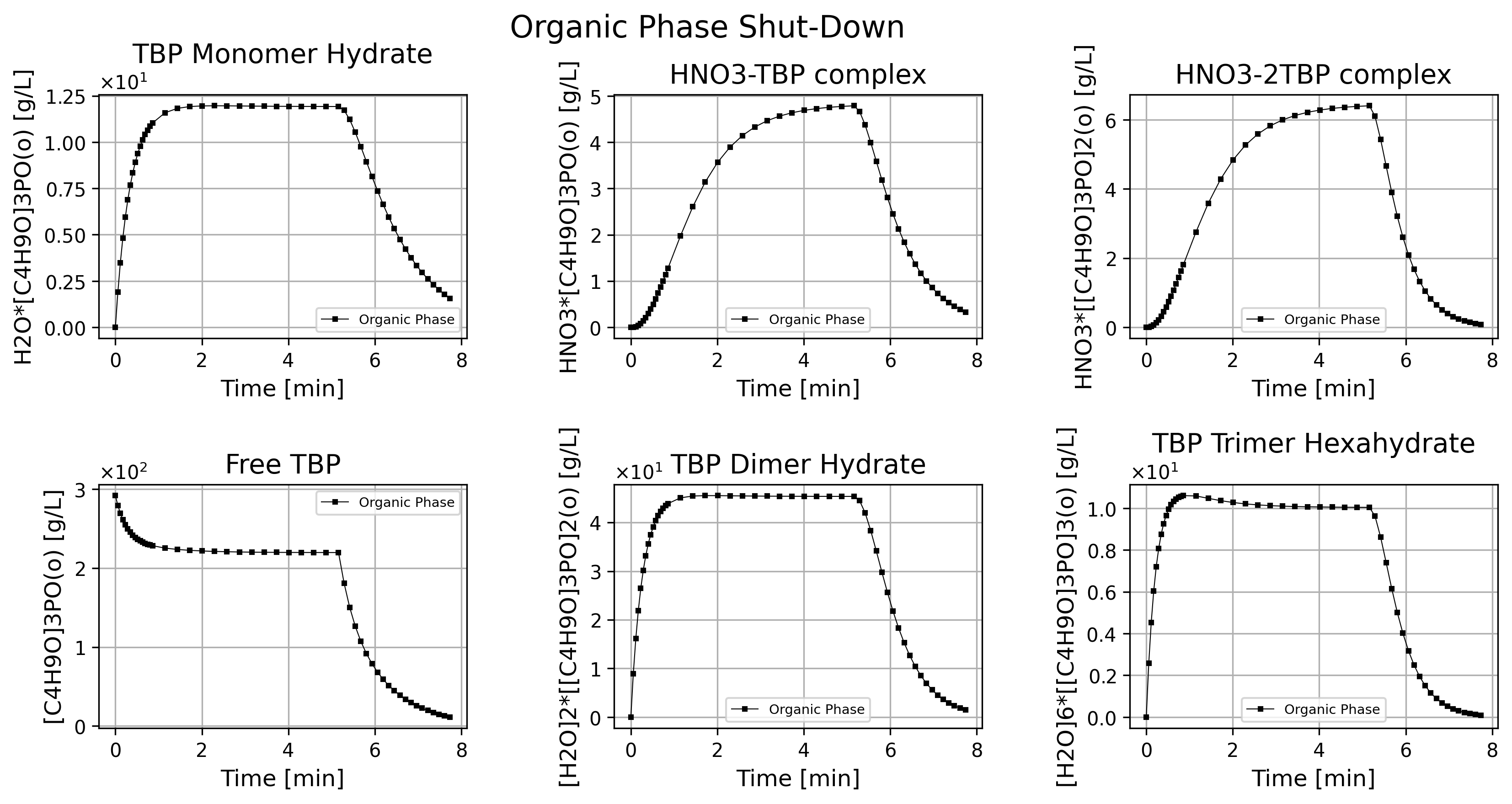
Figure 27: Organic phase species history dashboard at shut-down.
if cortix_ai:
    issues = ('+ Title your reponse as: Overview of the Organic Phase Data at Shut-Down.\n'
              f'+ Cover only the period after {round(stg.initial_time,2)} seconds when the concentration of TBP in the inflow is set to zero.'
    )
    cortix_ai.explain(phase=stg.organic_phase, issues=issues, markdown_header_level='<h4>', markdown_display=markdown_display, print_prompt=False, save_supporting_info=db_save)
Cortix AI assistant: working on explanation...
Overview of the Organic Phase Data at Shut-Down.
Data subset and timeframe
The analysis uses rows from time = 309.624 s through time = 464.436 s (inclusive), i.e., the 154.812 s period after the inflow TBP concentration is set to zero.
Key timestamp landmarks in this window: immediate post-shutdown sample at 309.624 s and final sample at 464.436 s.
Trends by species (values in g/L)
H₂O·[C₄H₉O]₃PO(o): 11.9203 -> 1.56691; absolute change −10.353 (−86.9%); monotonic decrease after 309.624 s.
HNO₃·[C₄H₉O]₃PO(o): 4.78878 -> 0.329669; absolute change −4.45911 (−93.1%); monotonic decrease.
HNO₃·[[C₄H₉O]₃PO]₂(o): 6.40608 -> 0.0840815; absolute change −6.3219985 (−98.7%); almost fully depleted by 464.436 s.
[C₄H₉O]₃PO(o) (TBP): 219.658 -> 11.2623; absolute change −208.3957 (−94.9%); large, rapid decline following shut-down.
[H₂O]₂·[[C₄H₉O]₃PO]₂(o): 45.3582 -> 1.46324; absolute change −43.89496 (−96.8%); steep, steady fall.
[H₂O]₆·[[C₄H₉O]₃PO]₃(o): 10.0384 -> 0.094421; absolute change −9.943979 (−99.1%); effectively removed by the end of the window.
Average rates over the shut-down period (309.624 -> 464.436 s, Δt = 154.812 s)
H₂O·[C₄H₉O]₃PO(o): −0.0669 g·L⁻¹·s⁻¹ (average).
HNO₃·[C₄H₉O]₃PO(o): −0.0288 g·L⁻¹·s⁻¹ (average).
HNO₃·[[C₄H₉O]₃PO]₂(o): −0.0408 g·L⁻¹·s⁻¹ (average).
[C₄H₉O]₃PO(o): −1.3456 g·L⁻¹·s⁻¹ (average).
[H₂O]₂·[[C₄H₉O]₃PO]₂(o): −0.2835 g·L⁻¹·s⁻¹ (average).
[H₂O]₆·[[C₄H₉O]₃PO]₃(o): −0.0643 g·L⁻¹·s⁻¹ (average).
Notable features and concise interpretation
Pre-shutdown behavior (prior to 309.624 s) shows near steady-state concentrations; the dataset shows a clear transition after 309.624 s consistent with shut-down of TBP inflow.
A rapid transient occurs immediately after 309.624 s (notably between 309.624 and 317.365 s): TBP drops sharply (≈ 17.7% drop in ~7.7 s), followed by continued monotonic decline of TBP and all complexes.
All organic-phase species are strongly depleted over the 154.8 s window: by 464.436 s TBP and complexes are reduced by ~95% or more (some complexes >98% removed).
Relative depletion ranking (largest fractional removal → smallest): HNO₃·[[C₄H₉O]₃PO]₂(o) ≈ [H₂O]₆·[[C₄H₉O]₃PO]₃(o) > [H₂O]₂·[[C₄H₉O]₃PO]₂(o) > HNO₃·[C₄H₉O]₃PO(o) > H₂O·[C₄H₉O]₃PO(o) ≈ [C₄H₉O]₃PO(o) (by absolute magnitude, TBP shows the largest absolute loss).
By the end of the record, complexed nitric acid and water species are near zero (substantially lower than initial post-shutdown levels), indicating the organic phase has been largely emptied or stripped of these solutes during the shut-down period.
AI Parameters:
+ LLM model (OpenAI) = gpt-5-mini
+ LLM cleverness     = 1.0
+ Total # of tokens  = 9526
'''Organic phase mass density'''
import matplotlib.pyplot as plt

quant = stg.mass_density_history('organic')

quant.plot(title='Organic Phase Mass Density @ %2.1f C Shut-Down'%unit.convert_temperature(stg_temperature,
           'K','C'), x_scaling=1/stg.flow_residence_time_avg, x_label=r'Time [$\bar{\tau}$]', y_label=quant.latex_name+r'$-\rho_\text{diluent}$'
           ' ['+quant.unit+']', show=True, figsize=[10,3], error_data=False)

fig_count += 1
print(f'Figure {fig_count}: Organic phase mass density history at shut-down.')
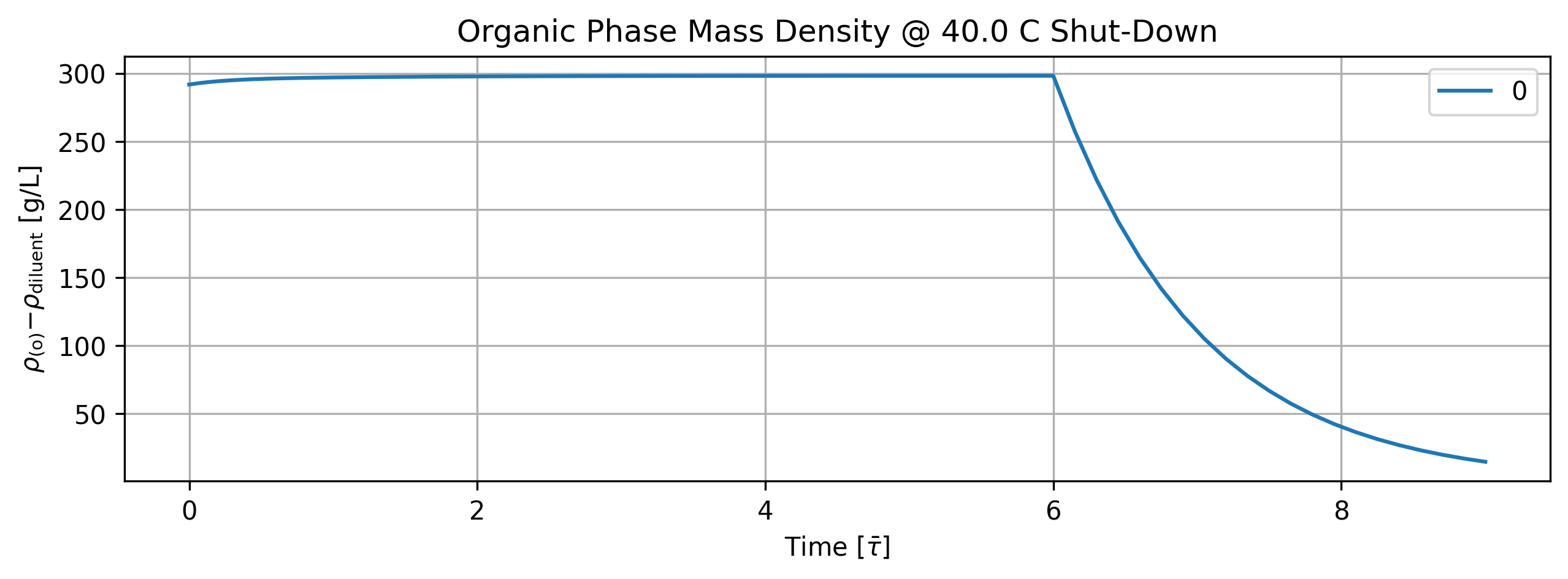
Figure 28: Organic phase mass density history at shut-down.
tbl_count += 1
print(f'Table {tbl_count}: Organic phase mass density history at shut-down.')
print('Time [s]  Organic Phase Mass Density [g/L]')
print(quant.value[::5].apply(lambda x: round(x,2)))
Table 17: Organic phase mass density history at shut-down.
Time [s]  Organic Phase Mass Density [g/L]
0.000000      291.75
17.201342     295.11
34.402683     296.35
51.604025     296.93
137.610734    297.91
223.617442    298.13
309.624151    298.17
348.327170    141.81
387.030188     66.83
425.733207     31.44
464.436226     14.80
Name: Organic Phase Mass Density [g/L]; Time History in [s], dtype: float64
1.7.2. Aqueous Phase Results#
'''Plot aqueous phase'''
# TODO: time axis normalized by phase flow residence time.
stg.aqueous_phase.plot(title='Aqueous Phase Shut-Down', legend='Aqueous Phase', nrows=2,ncols=3, show=True, figsize=[12,6])

fig_count += 1
print(f'Figure {fig_count}: Aqueous phase species history dashboard at shut-down.')
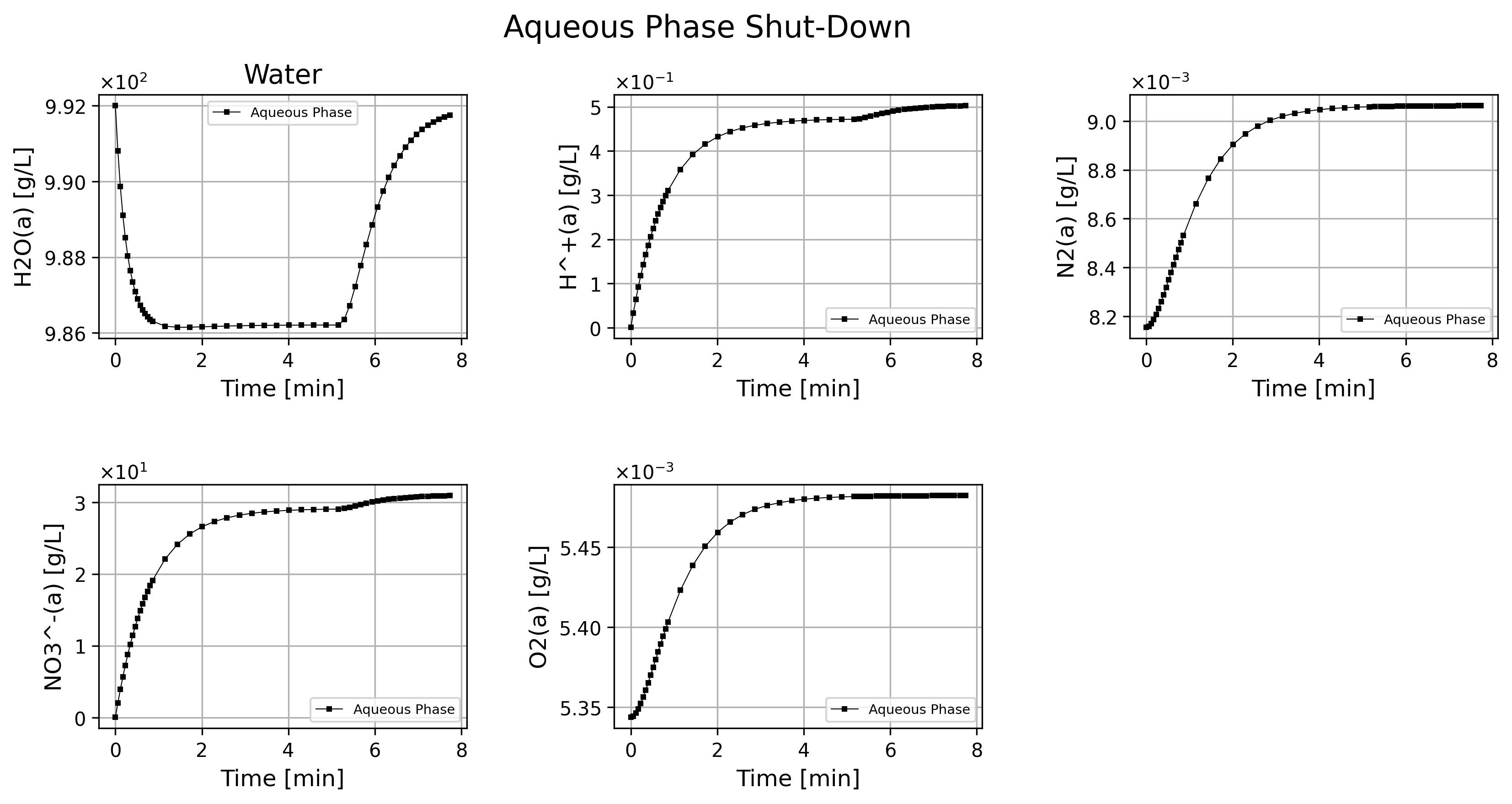
Figure 29: Aqueous phase species history dashboard at shut-down.
if cortix_ai:
    issues = ('+ Title your reponse as: Overview of the Aqueous Phase Data at Shut-Down.\n'
              f'+ Cover only the period after {round(stg.initial_time,2)} seconds when the concentration of TBP in the inflow is set to zero.'
    )
    cortix_ai.explain(phase=stg.aqueous_phase, issues=issues, markdown_header_level='<h4>', markdown_display=markdown_display, save_supporting_info=db_save)
Cortix AI assistant: working on explanation...
Overview of the Aqueous Phase Data at Shut-Down.
Data subset analyzed: t ≥ 309.624 s (first row at 309.624 s). Interval covered: 309.624 s → 464.436 s.
Summary of bulk magnitudes and dominant species
H₂O(a): bulk solvent, ~986.21 → 991.75 g/L (large absolute magnitude; ≈0.56% increase).
NO₃⁻(a): the largest dissolved solute, ~29.04 → 30.91 g/L (absolute increase ≈1.87 g/L; ≈6.44%).
H⁺(a): small absolute but notable relative change, ~0.4719 → 0.5023 g/L (Δ ≈ +0.0304 g/L; ≈6.44%).
N₂(a): ≈0.0090586 → 0.0090626 g/L (Δ ≈ +4.0×10⁻⁶ g/L; essentially constant).
O₂(a): ≈0.0054816 → 0.0054822 g/L (Δ ≈ +5.7×10⁻⁷ g/L; essentially constant).
Quantitative changes over 309.624 → 464.436 s (Δt = 154.812 s)
H₂O(a): +5.546 g/L; mean rate ≈ +0.0358 g·L⁻¹·s⁻¹.
NO₃⁻(a): +1.870 g/L; mean rate ≈ +0.0121 g·L⁻¹·s⁻¹.
H⁺(a): +0.03038 g/L; mean rate ≈ +1.96×10⁻⁴ g·L⁻¹·s⁻¹.
N₂(a): +3.98×10⁻⁶ g/L; mean rate ≈ +2.57×10⁻⁸ g·L⁻¹·s⁻¹.
O₂(a): +5.7×10⁻⁷ g/L; mean rate ≈ +3.68×10⁻⁹ g·L⁻¹·s⁻¹.
Trends and temporal behavior (detailed)
Monotonic increases: H₂O(a), H⁺(a) and NO₃⁻(a) all increase monotonically across the interval; increases are gradual but persistent.
Near-constant gases: N₂(a) and O₂(a) show only micro-scale rises (parts-per-million of their values) and are effectively constant for practical purposes.
Similar proportional change for H⁺ and NO₃⁻: both rise by ≈6.44% over the interval, indicating correlated relative increases (H⁺ absolute concentration remains small compared with NO₃⁻).
Rate behaviour: the averaged rates above are representative; short-windows inside the interval show modest acceleration in H₂O and NO₃⁻ (e.g., between ≈325–371 s values increase more rapidly than immediately after 309.6 s), but no reversal or strong transient is present.
Comparative remarks and significance
Mass/abundance hierarchy: H₂O(a) » NO₃⁻(a) ≫ H⁺(a) ≫ N₂(a), O₂(a).
The largest absolute change is in H₂O(a) (≈5.55 g/L) and NO₃⁻(a) (≈1.87 g/L); relative changes are largest for H⁺ and NO₃⁻ (both ≈6.44%).
Dissolved gases (N₂, O₂) remain negligible contributors to concentration change in this period.
Key numeric endpoints (start → end)
H₂O(a): 986.207 → 991.753 g/L
H⁺(a): 0.47187 → 0.502253 g/L
N₂(a): 0.00905861 → 0.00906259 g/L
NO₃⁻(a): 29.0439 → 30.9139 g/L
O₂(a): 0.00548158 → 0.00548215 g/L
Concise conclusion
After 309.624 s the aqueous phase displays steady increases in solvent (H₂O) and in dissolved NO₃⁻ and H⁺ (both ≈6.4% relative rise), while dissolved N₂ and O₂ remain essentially unchanged. The behavior is monotonic with modest acceleration mid-interval but no sign reversals.
AI Parameters:
+ LLM model (OpenAI) = gpt-5-mini
+ LLM cleverness     = 1.0
+ Total # of tokens  = 7518
'''Aqueous phase mass density'''
import matplotlib.pyplot as plt

quant = stg.mass_density_history('aqueous')

quant.plot(title='Aqueous Phase Mass Density @ %2.1f C Shut-Down'%unit.convert_temperature(stg_temperature,
           'K','C'), x_scaling=1/stg.flow_residence_time_avg, x_label=r'Time [$\bar{\tau}$]', y_label=quant.latex_name+
           ' ['+quant.unit+']', show=True, figsize=[10,3], error_data=False)

fig_count += 1
print(f'Figure {fig_count}: Aqueous phase mass density history at shut-down.')
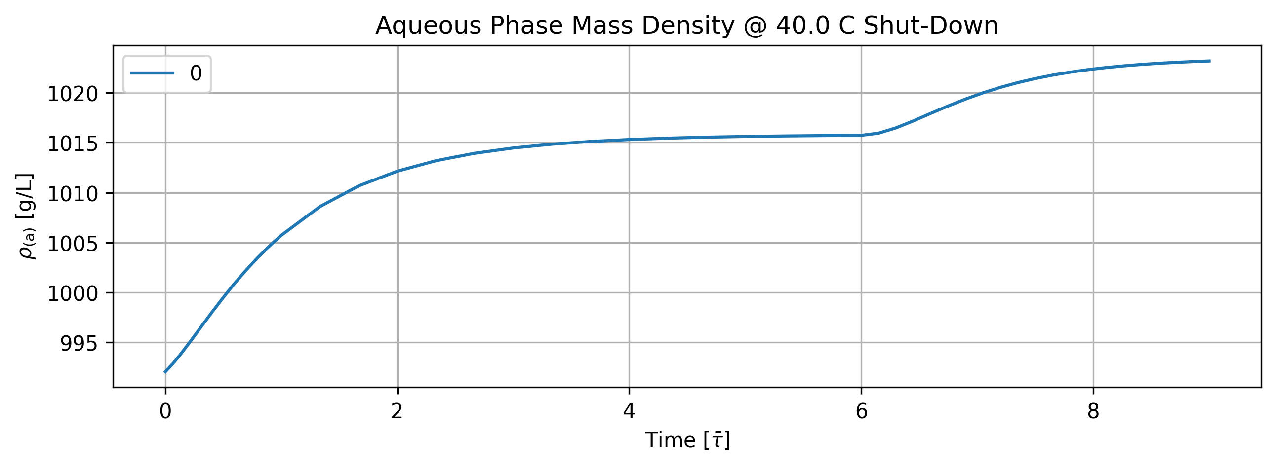
Figure 30: Aqueous phase mass density history at shut-down.
tbl_count += 1
print(f'Table {tbl_count}: Aqueous phase mass density history at shut-down.')
print('Time [s]  Aqueous Phase Mass Density [g/L]')
print(quant.value[::5].apply(lambda x: round(x,2)))
Table 18: Aqueous phase mass density history at shut-down.
Time [s]  Aqueous Phase Mass Density [g/L]
0.000000       992.08
17.201342      996.96
34.402683     1001.85
51.604025     1005.74
137.610734    1013.94
223.617442    1015.45
309.624151    1015.74
348.327170    1018.68
387.030188    1021.42
425.733207    1022.68
464.436226    1023.18
Name: Aqueous Phase Mass Density [g/L]; Time History in [s], dtype: float64
1.7.3. Vapor Phase Results#
'''Plot vapor phase'''
# TODO: time axis normalized by phase flow residence time.
stg.vapor_phase.plot(title='Vapor Phase Shut-Down', legend='Vapor Phase', nrows=2,ncols=3, show=True, figsize=[12,6])

fig_count += 1
print(f'Figure {fig_count}: Vapor phase species history dashboard at shut-down.')
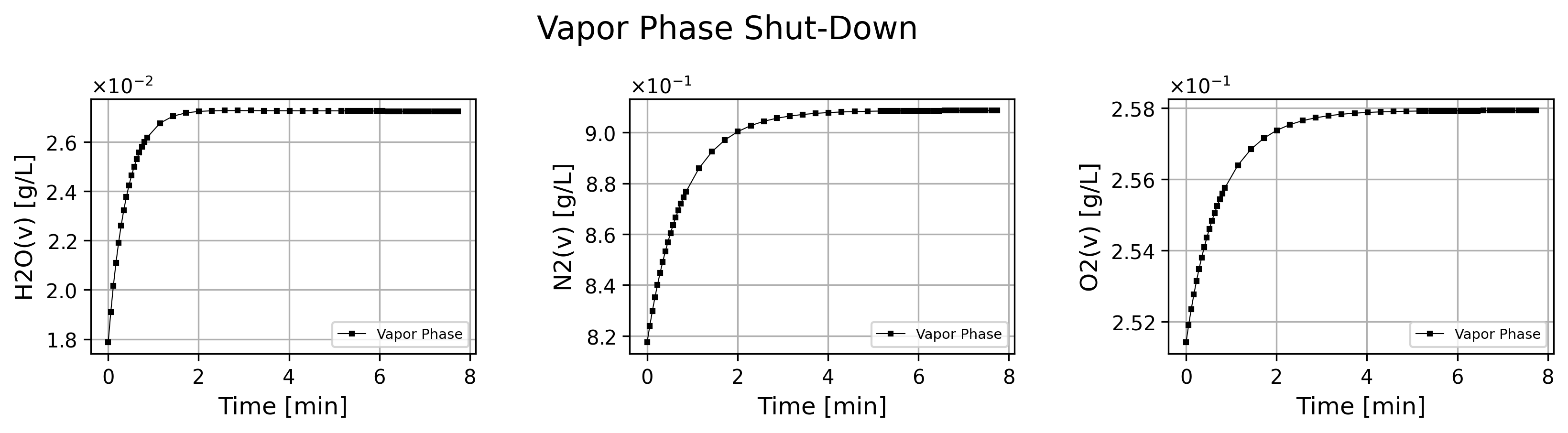
Figure 31: Vapor phase species history dashboard at shut-down.
if cortix_ai:
    issues = ('+ Title your reponse as: Overview of the Vapor Phase Data at Shut-Down.\n'
              f'+ Cover only the period after {round(stg.initial_time,2)} seconds when the concentration of TBP in the inflow is set to zero.'
    )
    cortix_ai.explain(phase=stg.vapor_phase, issues=issues, markdown_header_level='<h4>', markdown_display=markdown_display, save_supporting_info=db_save)
Cortix AI assistant: working on explanation...
Overview of the Vapor Phase Data at Shut-Down.
Scope
Period analyzed: t = 309.624 s through t = 464.436 s (Δt = 154.812 s). Only rows with time ≥ 309.624 s are considered; columns analyzed: time, H₂O(v), N₂(v), O₂(v).
Key numerical changes (start → end)
H₂O(v): 0.0272684 g/L → 0.0272443 g/L
Absolute change: −2.41×10⁻⁵ g/L
Relative change: −0.089% (approx)
Average rate: −1.56×10⁻⁷ g·L⁻¹·s⁻¹
N₂(v): 0.908398 g/L → 0.908598 g/L
Absolute change: +2.00×10⁻⁴ g/L
Relative change: +0.022% (approx)
Average rate: +1.29×10⁻⁶ g·L⁻¹·s⁻¹
O₂(v): 0.257921 g/L → 0.257934 g/L
Absolute change: +1.30×10⁻⁵ g/L
Relative change: +0.0050% (approx)
Average rate: +8.40×10⁻⁸ g·L⁻¹·s⁻¹
Trend comparison and interpretation
Magnitudes and ranking: N₂(v) ≫ O₂(v) ≫ H₂O(v) throughout the interval (final values ≈ 0.9086, 0.2579, 0.02725 g/L respectively).
Trends: after 309.624 s H₂O(v) shows a very small downward drift, while N₂(v) and O₂(v) show very small upward drifts.
Stability: all changes are extremely small (fractions of a percent) over 155 s, indicating the vapor composition is essentially quasi‑steady with slight slow drift following the TBP inflow cutoff.
Concise conclusion
In the post‑shut‑down interval the vapor phase is effectively steady: H₂O(v) decreases marginally, N₂(v) increases the most (but still only ~2×10⁻⁴ g/L), and O₂(v) increases negligibly. The composition changes are minute relative to absolute concentrations, consistent with approach to a new near‑steady state after TBP inflow is set to zero.
AI Parameters:
+ LLM model (OpenAI) = gpt-5-mini
+ LLM cleverness     = 1.0
+ Total # of tokens  = 5896
'''Vapor phase mass density'''
import matplotlib.pyplot as plt

quant = stg.mass_density_history('vapor')

quant.plot(title='Vapor Phase Mass Density @ %2.1f C Shut-Down'%unit.convert_temperature(stg_temperature,
           'K','C'), x_scaling=1/stg.flow_residence_time_avg, x_label=r'Time [$\bar{\tau}$]', y_label=quant.latex_name+
           ' ['+quant.unit+']', show=True, figsize=[10,3], error_data=False)

fig_count += 1
print(f'Figure {fig_count}: Vapor phase mass density history at shut-down.')
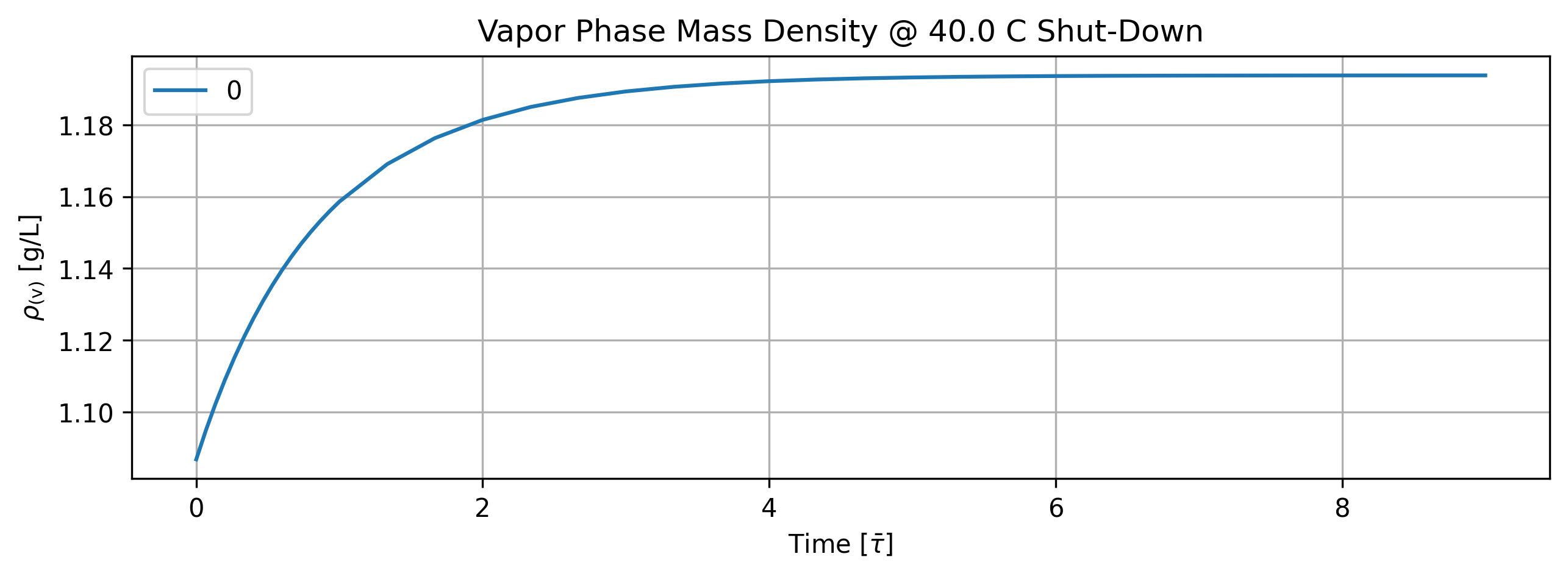
Figure 32: Vapor phase mass density history at shut-down.
tbl_count += 1
print(f'Table {tbl_count}: Vapor phase mass density history at shut-down.')
print('Time [s]  Vapor Phase Mass Density [g/L]')
print(quant.value[::5].apply(lambda x: round(x,2)))
Table 19: Vapor phase mass density history at shut-down.
Time [s]  Vapor Phase Mass Density [g/L]
0.000000      1.09
17.201342     1.12
34.402683     1.14
51.604025     1.16
137.610734    1.19
223.617442    1.19
309.624151    1.19
348.327170    1.19
387.030188    1.19
425.733207    1.19
464.436226    1.19
Name: Vapor Phase Mass Density [g/L]; Time History in [s], dtype: float64
1.7.3.1. Relative Humidity#
'''Compute relative humidity in the vapor phase'''
import matplotlib.pyplot as plt
from solvex import air_relative_humidity
from copy import deepcopy

h2o_vap_pd_series = deepcopy(stg.vapor_phase.df['H2O(v)'])
for idx, rho_h2o in enumerate(h2o_vap_pd_series):
    h2o_vap_pd_series.iloc[idx] = air_relative_humidity(stg_temperature, rho_h2o)
rh_pd_series = h2o_vap_pd_series
time_unit = stg.vapor_phase.time_unit
rh_pd_series.name = f'Relative Humidity History [{time_unit}]'

quant = Quantity(name=rh_pd_series.name, latex_name='RH', unit='%', info=f'Relative Humidity History (Vapor Phase) [{time_unit}]')
quant.value = h2o_vap_pd_series
quant.plot(title='Stage Rel. Humidity @ %2.1f C Shut-Down'%unit.convert_temperature(stg_temperature, 'K','C'),
           x_scaling=1/stg.flow_residence_time_avg, x_label=r'Time [$\bar{\tau}$]', y_label=quant.latex_name+' ['+quant.unit+']', show=True,
           figsize=[10,3])

fig_count += 1
print(f'Figure {fig_count}: Stage relative humidity history at shut-down.')
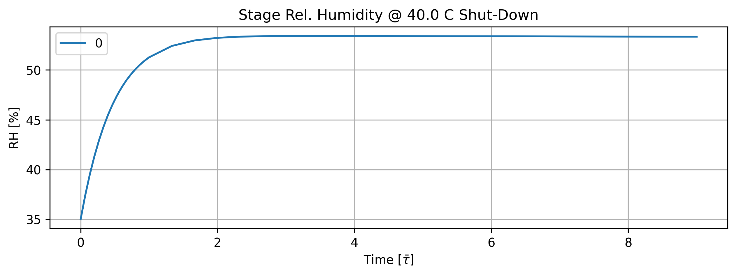
Figure 33: Stage relative humidity history at shut-down.
tbl_count += 1
print(f'Table {tbl_count}: Stage relative humidity history at shut-down.')
print('Time [s]  Rel. Humidity [%]')
print(quant.value.loc[n_startup::5].apply(lambda x: round(x,2)))
Table 20: Stage relative humidity history at shut-down.
Time [s]  Rel. Humidity [%]
17.201342     44.28
34.402683     48.95
51.604025     51.27
137.610734    53.40
223.617442    53.40
309.624151    53.39
348.327170    53.38
387.030188    53.36
425.733207    53.35
464.436226    53.34
Name: Relative Humidity History [s], dtype: float64
if cortix_ai:
    issues = ('+ Title your reponse as: Overview of the Relative Humidity Data at Shut-Down.\n'
              f'+ Cover only the period after {round(stg.initial_time,2)} seconds when the concentration of TBP in the inflow is set to zero.'
    )
    cortix_ai.explain(quant=quant, issues=issues, markdown_header_level='<h5>', markdown_display=markdown_display, print_prompt=False, save_supporting_info=db_save)
Cortix AI assistant: working on explanation...
Overview of the Relative Humidity Data at Shut-Down.
This analysis covers only the measurements at and after 309.624 s (the period after 309.62 s when TBP inflow concentration is set to zero): times 309.624 s, 356.068 s, 402.511 s, and 448.955 s. The second column is Relative Humidity (vapor phase) reported in percent [%].
Data included
Time [s]: 309.624, 356.068, 402.511, 448.955.
Relative Humidity [%]: 53.3908, 53.3765, 53.3563, 53.3456.
Sampling cadence
Inter-measurement intervals are uniform in this period: each step is ≈ 46.444 s (309.624 -> 356.068 -> 402.511 -> 448.955).
Descriptive statistics (n = 4)
Mean RH ≈ 53.3673 %.
Minimum RH = 53.3456 %, Maximum RH = 53.3908 %.
Range = 0.0452 percentage points.
Standard deviation (population) ≈ 0.0175 % (sample standard deviation ≈ 0.0203 %).
Trend over the period
Absolute change from 309.624 s to 448.955 s: −0.0452 percentage points (53.3908 % -> 53.3456 %).
Time span: 139.331 s.
Mean rate of change ≈ −0.0003245 %/s (≈ −1.17 %/hour), indicating a very small, gradual decrease in RH after shut-down.
Rates between successive measurements
309.624 -> 356.068 (Δt = 46.444 s): ΔRH = −0.0143 -> rate ≈ −0.0003079 %/s (≈ −1.11 %/hr).
356.068 -> 402.511 (Δt = 46.443 s): ΔRH = −0.0202 -> rate ≈ −0.0004349 %/s (≈ −1.57 %/hr).
402.511 -> 448.955 (Δt = 46.444 s): ΔRH = −0.0107 -> rate ≈ −0.0002304 %/s (≈ −0.83 %/hr).
Brief interpretation
After TBP inflow is set to zero, the vapor-phase relative humidity remains essentially steady with a very small downward drift (total drop ~0.045 % over ~139 s). Variability is minor (std dev ≈ 0.018 %), and the short-term rates fluctuate modestly around the small negative mean trend.
AI Parameters:
+ LLM model (OpenAI) = gpt-5-mini
+ LLM cleverness     = 1.0
+ Total # of tokens  = 4771
1.7.4. Reaction Rate Density#
This quantity only makes sense per volume of the mixture.
'''Reaction rate density'''
import matplotlib.pyplot as plt

quant = stg.r_vec_history()
quant.plot(title='Reaction Rate Density @ %2.1f C Shut-Down'%unit.convert_temperature(stg_temperature,
           'K','C'), x_scaling=1/stg.flow_residence_time_avg, x_label=r'Time [$\bar{\tau}$]', y_label=quant.latex_name+
           ' ['+quant.unit+']', legend=stg.rxn_mech.reactions, show=True, figsize=[10,3], error_data=False)

fig_count += 1
print(f'Figure {fig_count}: Reaction rate density history at shut-down.')
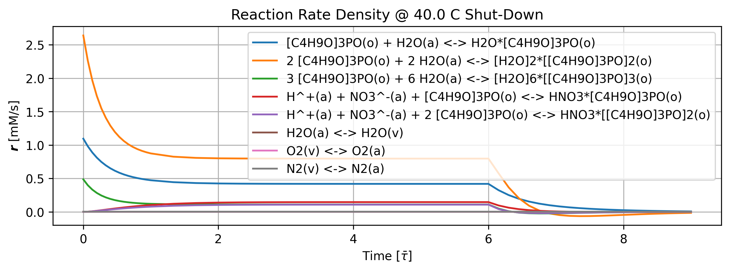
Figure 34: Reaction rate density history at shut-down.
if cortix_ai:
    issues = ('+ Title your reponse as: Overview of Reaction Rates Density at Shut-Down.\n'
              f'+ Cover only the period after {round(stg.initial_time,2)} seconds when the concentration of TBP in the inflow is set to zero.'
    )
    cortix_ai.explain(quant=quant, issues=issues, markdown_header_level='<h4>', markdown_display=markdown_display, print_prompt=False, save_supporting_info=db_save)
Cortix AI assistant: working on explanation...
Overview of Reaction Rates Density at Shut-Down.
Data subset and context: the table rows used are the four times after TBP inflow is set to zero (t = 309.624 s, 356.068 s, 402.511 s, 448.955 s). Units: reaction-rate density [mM/s]. Reactions (indices 0→7) are:
0: [C₄H₉O]₃PO(o) + H₂O(a) <-> H₂O·[C₄H₉O]₃PO(o)
1: 2 [C₄H₉O]₃PO(o) + 2 H₂O(a) <-> [H₂O]₂·[[C₄H₉O]₃PO]₂(o)
2: 3 [C₄H₉O]₃PO(o) + 6 H₂O(a) <-> [H₂O]₆·[[C₄H₉O]₃PO]₃(o)
3: H⁺(a) + NO₃⁻(a) + [C₄H₉O]₃PO(o) <-> HNO₃·[C₄H₉O]₃PO(o)
4: H⁺(a) + NO₃⁻(a) + 2 [C₄H₉O]₃PO(o) <-> HNO₃·[[C₄H₉O]₃PO]₂(o)
5: H₂O(a) <-> H₂O(v)
6: O₂(v) <-> O₂(a)
7: N₂(v) <-> N₂(a)
Overall trend after shut-down: TBP-related reaction rates (indices 0–4) drop rapidly toward zero within the first interval after 309.624 s and in most cases cross sign to small negative values (net consumption) or settle near zero; phase-exchange reactions (indices 5–7) remain essentially unchanged at small positive rates.
Timescale and magnitude of the primary response:
The largest changes occur between 309.624 s and 356.068 s (≈46 s after shut-down), indicating a fast system response to removal of TBP in the inflow.
By 448.955 s the TBP-related rates are all ≈0 (magnitudes ≤ 0.011 mM/s, typically ≪0.1 mM/s), i.e., reduced by ≈97–103% relative to their values at 309.624 s.
Per-reaction behavior (values are [mM/s] at t = 309.624 → 356.068 → 402.511 → 448.955; delta = final − initial):
0 ([C₄H₉O]₃PO + H₂O <-> H₂O·[C₄H₉O]₃PO): 0.419134 → 0.100141 → 0.0325229 → 0.0107605; delta = −0.408374 (≈ −97.4%) — large positive production rate falls toward zero.
1 (dimer hydration): 0.797538 → −0.0228233 → −0.0533838 → −0.0210582; delta = −0.818596 (sign flip to small net consumption; magnitude reduced to ≈0.02).
2 (trimer hydration): 0.110605 → −0.0229238 → −0.00770646 → −0.00166123; delta = −0.112266 (small negative residual, approaching zero).
3 (HNO₃·TBP formation, monomer): 0.14649 → 0.010132 → −0.000994863 → −0.00091144; delta = −0.147401 (drops to essentially zero with minor sign crossing).
4 (HNO₃·TBP formation, dimer): 0.108296 → −0.0184433 → −0.00690328 → −0.00173299; delta = −0.110029 (small negative residual trending to zero).
5 (H₂O(a) <-> H₂O(v)): 0.00133096 → 0.00132988 → 0.00132952 → 0.00132949; delta = −1.47e−06 (essentially constant small positive flux).
6 (O₂(v) <-> O₂(a)): 0.0014277 → 0.0014277 → 0.0014277 → 0.0014277; delta = 0.0 (no detectable change in these records).
7 (N₂(v) <-> N₂(a)): 0.00269596 → 0.00269596 → 0.00269596 → 0.00269596; delta = 0.0 (no detectable change).
Key observations and implications:
Shutdown of TBP feed produces an immediate, large reduction in TBP-associated reaction-rate densities (indices 0–4); most rates go from clear positive production to values near zero or slight net consumption within ~50 s.
Gas/solvent phase-exchange processes (indices 5–7) are effectively decoupled from the TBP shut-down on the shown timescale and remain nearly constant small positive fluxes.
By the last sampled time (448.955 s) all TBP-related reaction rates are reduced by two orders of magnitude or more compared with their pre-shutdown values, indicating that production/formation pathways for TBP-containing species have essentially ceased in this time window.
AI Parameters:
+ LLM model (OpenAI) = gpt-5-mini
+ LLM cleverness     = 1.0
+ Total # of tokens  = 6962
1.7.5. Species Generation Rate Density#
This quantity is on the basis of mixing volume so all species generation values can be compared.
'''Species generation rate density'''
import matplotlib.pyplot as plt

quant = stg.g_vec_history()
quant.plot(title='Species Generation Rate Density @ %2.1f C Shut-Down'%unit.convert_temperature(stg_temperature,
           'K','C'), x_scaling=1/stg.flow_residence_time_avg, x_label=r'Time [$\bar{\tau}$]', y_label=quant.latex_name+
           ' ['+quant.unit+']', legend=stg.rxn_mech.species_names, show=True, figsize=[10,3], error_data=False)

fig_count += 1
print(f'Figure {fig_count}: Species generation rate density history at shut-down.')
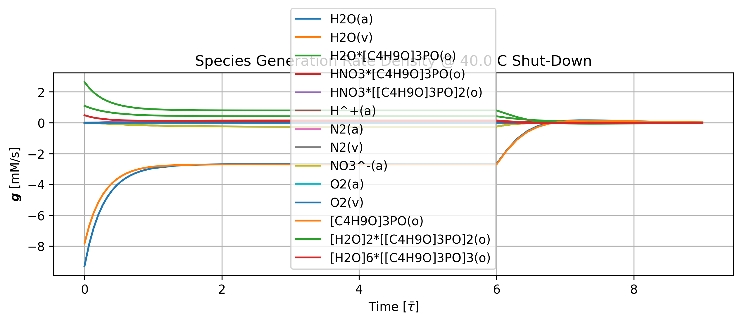
Figure 35: Species generation rate density history at shut-down.
if cortix_ai:
    issues = ('+ Title your reponse as: Overview of Species Generation Rates Density at Shut-Down.\n'
              f'+ Cover only the period after {round(stg.initial_time,2)} seconds when the concentration of TBP in the inflow is set to zero.'
    )
    cortix_ai.explain(quant=quant, issues=issues, markdown_header_level='<h4>', markdown_display=markdown_display, print_prompt=False, save_supporting_info=db_save)
Cortix AI assistant: working on explanation...
Overview of Species Generation Rates Density at Shut-Down.
Period covered: t ≥ 309.624 s (rows at 309.624, 356.068, 402.511, 448.955 s). All values are generation-rate densities in mM/s.
Concise summary
The moment of TBP inflow shut‑off (309.624 s) is associated with large negative generation rates for free TBP ([C₄H₉O]₃PO(o)) and liquid H₂O(a), and large positive rates for several TBP–water adducts; within ~140 s after shut‑down these large rates collapse toward small magnitudes (near zero or small sign changes), indicating rapid re-equilibration of TBP-related species.
Simple gases N₂ and O₂ (both aqueous and vapor entries) show essentially constant, small rates across the period (no transient response).
The highest-magnitude transient terms are: H₂O(a) and [C₄H₉O]₃PO(o) at shut‑off, and the dimer/trimer TBP–water adducts that are produced at shut‑off and then decline toward small negative or near‑zero rates.
Per-species observations (ordered as provided)
H₂O(a): -2.67917 at 309.624 -> 0.0817182 at 356.068 -> 0.119154 at 402.511 -> 0.0399937 at 448.955; strong consumption at shut‑off reverses to small production and then decays toward zero.
H₂O(v): 0.00133096 -> 0.00132988 -> 0.00132952 -> 0.00132949; positive, essentially constant (~1.33×10⁻³ mM/s).
H₂O·[C₄H₉O]₃PO(o): 0.419134 -> 0.100141 -> 0.0325229 -> 0.0107605; sizable production at shut‑off that rapidly decreases toward zero (monotonic decay).
HNO₃·[C₄H₉O]₃PO(o): 0.14649 -> 0.010132 -> -0.000994863 -> -0.00091144; small positive at shut‑off that falls through zero to a small net consumption.
HNO₃·[[C₄H₉O]₃PO]₂(o): 0.108296 -> -0.0184433 -> -0.00690328 -> -0.00173299; production at shut‑off followed by net consumption (negative) that relaxes toward zero.
H⁺(a): -0.254786 -> 0.0083113 -> 0.00789814 -> 0.00264443; large consumption at shut‑off flips to small production and then declines toward zero.
N₂(a): 0.00269596 -> 0.00269596 -> 0.00269596 -> 0.00269596; constant small production (no discernible transient).
N₂(v): -0.00269596 -> -0.00269596 -> -0.00269596 -> -0.00269596; constant small consumption in vapor form (mirror of N₂(a)).
NO₃⁻(a): -0.254786 -> 0.0083113 -> 0.00789814 -> 0.00264443; identical pattern to H⁺(a) (large consumption at shut‑off then small production → decay).
O₂(a): 0.0014277 -> 0.0014277 -> 0.0014277 -> 0.0014277; constant small production.
O₂(v): -0.0014277 -> -0.0014277 -> -0.0014277 -> -0.0014277; constant small consumption (vapor), mirror of O₂(a).
[C₄H₉O]₃PO(o): -2.7091 -> 0.0410312 -> 0.112165 -> 0.0407169; very large consumption at shut‑off (−2.7091 mM/s) reverses to small positive generation and then relaxes toward a small positive value.
[H₂O]₂·[[C₄H₉O]₃PO]₂(o): 0.797538 -> -0.0228233 -> -0.0533838 -> -0.0210582; strong production at shut‑off is quickly lost and turns into small net consumption that trends back toward zero.
[H₂O]₆·[[C₄H₉O]₃PO]₃(o): 0.110605 -> -0.0229238 -> -0.00770646 -> -0.00166123; moderate production at shut‑off then small negative generation tending to zero.
Brief quantitative note
Largest absolute changes occur at the instant of shut‑off (309.624 s): [C₄H₉O]₃PO(o) ≈ −2.709 mM/s and H₂O(a) ≈ −2.679 mM/s, and the dimer adduct [H₂O]₂·[[C₄H₉O]₃PO]₂(o) ≈ +0.798 mM/s. By 356–449 s these magnitudes have fallen by roughly one to two orders of magnitude for most species, with many rates near ±10⁻³–10⁻² mM/s.
AI Parameters:
+ LLM model (OpenAI) = gpt-5-mini
+ LLM cleverness     = 1.0
+ Total # of tokens  = 7350
1.7.6. Mass Balance Residual#
This is actually the total mass generation rate density (mixing volume) residual; a small number in view of total mass conservation.
'''Mass balance residuals'''
import matplotlib.pyplot as plt

quant = stg.mass_balance_residual_history()
quant.plot(title='Total Mass Generation Rate Density @ %2.1f C Shut-Down'%unit.convert_temperature(stg_temperature,
           'K','C'), x_scaling=1/stg.flow_residence_time_avg, x_label=r'Time [$\bar{\tau}$]', y_label=quant.latex_name+
           ' ['+quant.unit+']', markers_only=True, legend=['Residual'], show=True, figsize=[10,3])

fig_count += 1
print(f'Figure {fig_count}: Total mass generation rate density residual history at shut-down.')
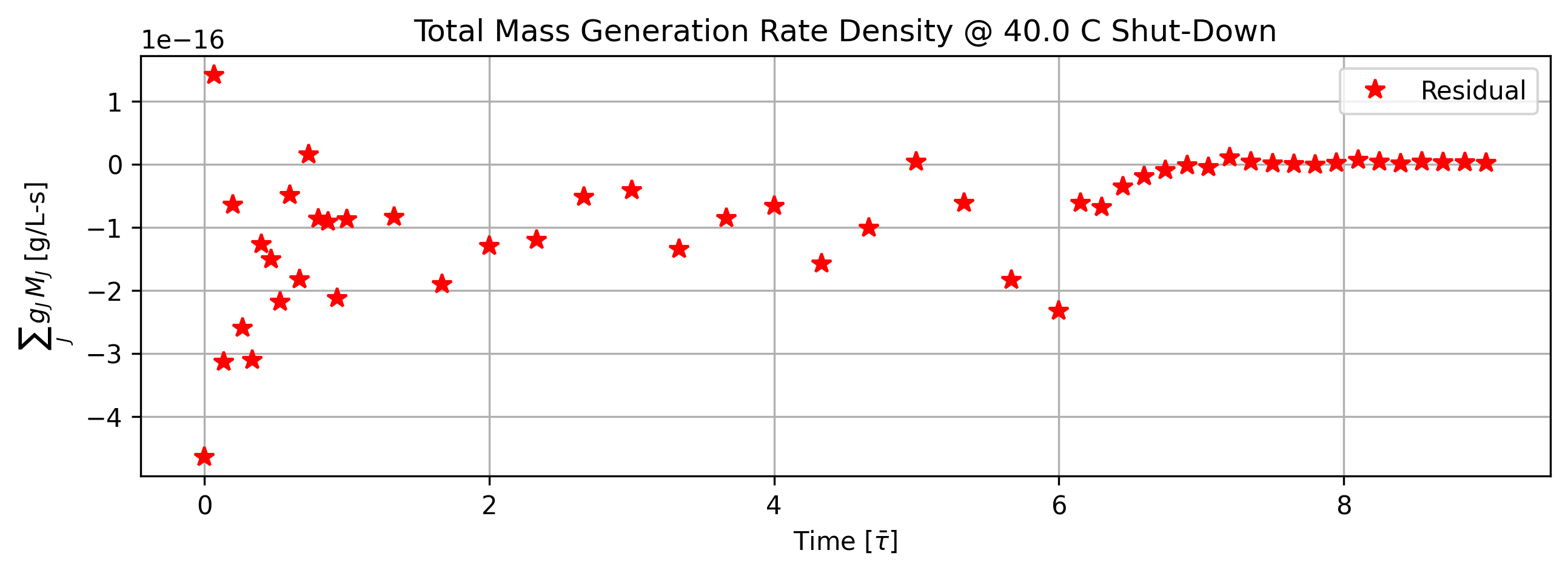
Figure 36: Total mass generation rate density residual history at shut-down.
if cortix_ai:
    issues = ('+ Title your reponse as: Total Mass Generation Rate Density Residual at Shut-Down.\n'
             f'+ Cover only the period after {round(stg.initial_time,2)} seconds when the concentration of TBP in the inflow is set to zero.'
    )
    cortix_ai.explain(quant=quant, issues=issues, markdown_header_level='<h4>', markdown_display=markdown_display, print_prompt=False, save_supporting_info=db_save)
Cortix AI assistant: working on explanation...
Total Mass Generation Rate Density Residual at Shut-Down.
After TBP in the inflow is set to zero (t ≥ 309.624 s), the table provides the total mass generation rate density (units: g/L-s) in the mixing volume at four times; the following summarizes and interprets those values.
Observations: at 309.624 s the residual is -2.32832e-16 g/L-s; at 356.068 s it is -1.87025e-18 g/L-s; at 402.511 s it is -1.22650e-18 g/L-s; at 448.955 s it is 2.31071e-18 g/L-s.
Time column analysis: the four samples after shut-down are at roughly 309.6 s, 356.1 s, 402.5 s, and 449.0 s, sampling the post-shut-down transient up to ≈449 s.
Magnitude and sign behavior: the largest magnitude residual occurs immediately after shut-down (≈2.33×10⁻¹⁶ g/L-s, negative); the subsequent three values are O(10⁻¹⁸) and include both small negative and positive signs, i.e., they cross zero.
Summary statistics (post-shut-down subset): mean ≈ -5.84×10⁻¹⁷ g/L-s; population standard deviation ≈ 1.01×10⁻¹⁶ g/L-s; maximum absolute value ≈ 2.33×10⁻¹⁶ g/L-s.
Interpretation: all residuals are effectively zero within numerical round-off; the sign changes and O(10⁻¹⁸–10⁻¹⁶) magnitudes indicate numerical noise rather than physical mass production or consumption. Mass balance in the mixing volume is therefore conserved to within ~10⁻¹⁶ g/L-s over the sampled post-shut-down period.
Practical takeaway: for the period after TBP inflow goes to zero, the total mass generation rate density shows no physically meaningful net generation or loss; the reported values quantify the residual numerical error scale.
AI Parameters:
+ LLM model (OpenAI) = gpt-5-mini
+ LLM cleverness     = 1.0
+ Total # of tokens  = 4030
1.8. AI Reports#
The Stage AI Report agent builds a Knowledge Base from the simulation up to this point, and uses it as a retrieval augmented generation (RAG) AI to analyze the results and provide a report.
'''Create and Configure a StageAI Object for a particular stg'''
if stage_ai:
    from stage_ai import StageAI
    stage_ai = StageAI(stg, llm_model='gpt-5-mini', llm_cleverness=0.8)
    stage_ai.n_chunks = 8
    stage_ai.markdown_header_level = '<h4>'
1.8.1. Aqueous Phase#
Request a report from the LLM.
if stage_ai:
    issues = ('+ Title your response as: Aqueous Phase Analysis.\n'
              '+ Discuss in particular, for the aqueous phase, why the simulated steady-state concentration of O2 in the aqueous'
              ' phase is lower than N2 when the solubility of O2 in the aqueous phase is higher than the solubility of N2.\n'
              f'+ Consider stage efficiency only up to {round(stg.initial_time,2)} seconds.'
             )
    stage_ai.report(phase='aqueous', issues=issues, markdown_display=markdown_display, print_prompt=False, save_supporting_info=db_save)
Stage AI assistant: working on report...
Aqueous Phase Analysis
Introduction
This report analyzes the aqueous phase in the provided Stage Knowledge Base (source: stg.aqueous_phase). The system is a multi-phase (aqueous-organic-vapor) mixing system. Analysis focuses on aqueous-phase species, their time histories (mass concentration, g/L), stage efficiency up to 309.62 s, reaction mechanisms that involve the aqueous phase, and an explanation for why the simulated steady-state aqueous O₂ concentration (mass basis) is lower than N₂ despite O₂ having higher intrinsic solubility. Stage information is present and used (“stage”).
Species characteristics (aqueous-phase relevant)
Table: Commercial name and chemical formula with key characteristics (molar mass, phase). All molar masses in kg/mol, rounded to 5 significant digits.
| Commercial name | Chemical formula | Phase | Molar mass (kg/mol) | |—|—:|—|—:| | Water | H₂O(a) | aqueous phase | 0.018015 | | Proton (Hydrogen ion) | H⁺(a) | aqueous phase | 0.0010074 | | Nitrogen | N₂(a) | aqueous phase | 0.028013 | | Nitrate (ion) | NO₃⁻(a) | aqueous phase | 0.062006 | | Oxygen | O₂(a) | aqueous phase | 0.031999 |
Time-dependent aqueous-phase species (mass concentrations)
Table: Time series of aqueous-phase mass concentrations. Units: g/L for concentrations, seconds (s) for time. Values rounded to 5 significant digits.
| Time (s) | Water, H₂O(a) (g/L) | Proton, H⁺(a) (g/L) | Nitrogen, N₂(a) (g/L) | Nitrate, NO₃⁻(a) (g/L) | Oxygen, O₂(a) (g/L) | |—:|—:|—:|—:|—:|—:| | 0.0000 | 992.00 | 0.0010074 | 0.0081544 | 0.062006 | 0.0053437 | | 20.640 | 987.65 | 0.16531 | 0.0082590 | 10.175 | 0.0053606 | | 41.280 | 986.50 | 0.27209 | 0.0084418 | 16.747 | 0.0053894 | | 103.21 | 986.15 | 0.41544 | 0.0088442 | 25.571 | 0.0054504 | | 206.42 | 986.20 | 0.46530 | 0.0090319 | 28.639 | 0.0054778 | | 309.62 | 986.21 | 0.47187 | 0.0090586 | 29.044 | 0.0054816 | | 356.07 | 988.86 | 0.48762 | 0.0090611 | 30.013 | 0.0054819 | | 402.51 | 990.90 | 0.49788 | 0.0090621 | 30.645 | 0.0054821 | | 448.96 | 991.64 | 0.50166 | 0.0090625 | 30.877 | 0.0054821 |
Stage efficiency (considered up to 309.62 s)
Table: Stage overall efficiency (mean ± std) in percent. Time units in seconds. Only timestamps ≤ 309.62 s are used for claims about equilibrium.
| Time (s) | Mean efficiency (%) | Std dev (%) | |—:|—:|—:| | 0.0000 | 16.880 | 22.210 | | 20.640 | 33.060 | 13.590 | | 41.280 | 41.140 | 10.440 | | 103.21 | 48.170 | 4.4400 | | 206.42 | 50.220 | 1.6500 | | 309.62 | 50.490 | 1.4400 |
Notes:
Stage mass balance residual (Total Mass Generation Rate Density [g/L-s]) is available at the same timestamps and is effectively zero (values reported as -0.0 or 0.0), indicating no detectable net mass generation in the stage-level residuals provided.
Reaction mechanism (reactions that involve the aqueous phase)
Only reactions that explicitly include aqueous-phase species are listed and analyzed. For each reaction I provide the reaction expression (using UTF-8 subscripts/superscripts where applicable), the Stage Knowledge Base description text (information content), and an extra explanatory sub-item describing the mechanistic role.
Reaction 1:
[C₄H₉O]₃PO(o) + H₂O(a) <-> H₂O*[C₄H₉O]₃PO(o)
Description (from KB): complexation of one H2O molecule
Additional information: This reaction is the mono-complexation (binding) of a single aqueous H₂O molecule by tributyl phosphate (TBP) in the organic phase; it represents transfer/association of an aqueous water molecule into an organic TBP-associated species (phase involvement: aqueous and organic). The aqueous phase species involved is H₂O(a).
Reaction 2:
2 [C₄H₉O]₃PO(o) + 2 H₂O(a) <-> [H₂O]₂*[[C₄H₉O]₃PO]₂(o)
Description (from KB): complexation of two H2O molecules
Additional information: This is a higher-order complexation: two TBP molecules coordinate two aqueous H₂O molecules into an organic-phase complex. It models progressive solvation/entrainment of aqueous water into organic TBP clusters. The aqueous phase species are H₂O(a).
Reaction 3:
3 [C₄H₉O]₃PO(o) + 6 H₂O(a) <-> [H₂O]₆*[[C₄H₉O]₃PO]₃(o)
Description (from KB): complexation of six H2O molecules
Additional information: Even larger TBP-water aggregates are represented here (three TBP molecules complexing six H₂O). This again couples aqueous water to organic-phase complexes and can change aqueous water activity locally.
Reaction 4:
H⁺(a) + NO₃⁻(a) + [C₄H₉O]₃PO(o) <-> HNO₃*[C₄H₉O]₃PO(o)
Description (from KB): one TBP complexation of HNO3
Additional information: This reaction describes extraction/complexation of aqueous nitric acid (represented as H⁺(a) + NO₃⁻(a)) by a single TBP molecule into an organic-phase TBP–HNO₃ complex. It couples aqueous ionic species (H⁺, NO₃⁻) to organic-phase extraction and affects aqueous acidity and nitrate concentration.
Reaction 5:
H⁺(a) + NO₃⁻(a) + 2 [C₄H₉O]₃PO(o) <-> HNO₃*[[C₄H₉O]₃PO]₂(o)
Description (from KB): two TBP complexation of HNO3
Additional information: Similar to Reaction 4 but with two TBP molecules forming a larger organic extract of HNO₃. This further reduces aqueous free H⁺ and NO₃⁻ when forward, and can change aqueous pH and nitrate distribution.
Reaction 6:
H₂O(a) <-> H₂O(v)
Description (from KB): H2O vaporization in air
Additional information: This is the aqueous–vapor phase exchange (evaporation/condensation) of water; it directly couples aqueous H₂O to vapor-phase H₂O and is a mass-transfer process, not a chemical transformation.
Reaction 7:
O₂(v) <-> O₂(a)
Description (from KB): O2 aeration of aqueous phase
Additional information: Gas–liquid exchange of oxygen between vapor and aqueous phases (aeration). The exchange rate (kinetics) and gas-phase partial pressure determine how O₂ accumulates in the aqueous phase.
Reaction 8:
N₂(v) <-> N₂(a)
Description (from KB): N2 aeration of aqueous phase
Additional information: Gas–liquid exchange of nitrogen between vapor and aqueous phases. As with O₂, kinetics and vapor-phase composition control N₂ uptake.
Comments on reaction mechanism involving the aqueous phase
The aqueous-phase reactions include two broad categories:
Extraction/complexation processes: TBP (organic) complexes with aqueous H₂O and aqueous ionic species (H⁺, NO₃⁻) and forms organic-phase complexes. These deplete aqueous H₂O, H⁺ and NO₃⁻ depending on direction and kinetics.
Gas–liquid mass transfer: H₂O, O₂ and N₂ exchange between vapor and aqueous phases; these are reversible transfer processes that are controlled by interfacial transfer rates and the gas-phase partial pressures/compositions.
The KB does not show explicit chemical reactions that consume O₂(a) or N₂(a) within the aqueous phase (no aqueous oxidation reactions listed). Therefore net aqueous changes for O₂ and N₂ are controlled by their gas–liquid exchange reactions (Reactions 7 and 8) plus any transport limitations or coupling to other processes (e.g., changing water activity, complexation indirectly altering solubility).
Why simulated steady-state O₂(a) (g/L) is lower than N₂(a) despite O₂ having higher solubility
Key points (supported by KB data and reaction set):
Non-equilibrium (stage efficiency):
The stage overall efficiency up to 309.62 s is ~50% (mean ≈ 50.49% at 309.62 s) with non-negligible standard deviations. Because stage efficiency is well below ~100%, the stage is not at chemical/thermodynamic equilibrium. Therefore measured steady-state concentrations at these times are kinetic or operational steady states, not thermodynamic equilibrium values. Mass-transfer kinetics and imperfect stage operation can maintain concentrations that differ from equilibrium predictions.
Gas-phase driving force (partial pressure / composition) and transfer kinetics:
The equilibrium aqueous concentration of a dissolved gas depends on both solubility (Henry-type behavior) and the gas-phase partial pressure. If the gas-phase mole fraction (partial pressure) of N₂ is substantially larger than that of O₂ (typical air composition: N₂ ~78%, O₂ ~21%), the higher driving force for N₂ dissolution may offset its lower intrinsic solubility and produce a higher aqueous concentration of N₂.
The KB does not provide explicit gas-phase compositions, but the presence of aeration exchange reactions (O₂(v) <-> O₂(a) and N₂(v) <-> N₂(a)) means aqueous concentrations are governed by gas-phase partial pressures and transfer kinetics. If the gas-phase N₂ partial pressure or supply is larger, N₂(a) can end up higher.
Units (mass concentration, g/L) and molar mass effects:
The KB concentrations are given in g/L (mass basis). Because N₂ has slightly lower molar mass (0.028013 kg/mol) than O₂ (0.031999 kg/mol), differences in molar concentrations appear when converted to g/L; however, the KB shows N₂ molar concentration is still larger than O₂ molar concentration (i.e., not solely a molar-mass artifact). Converting the provided g/L values to mol/L confirms N₂(a) > O₂(a) in molar terms at the reported times.
Initial conditions and system dynamics:
The initial aqueous values (t = 0 s) already show N₂(a) > O₂(a). With stage efficiency < 100% and the extraction/complexation processes present (that can alter water activity and interfacial mass transfer), the system can remain in a non-equilibrium steady state where N₂ remains more concentrated than O₂ in the aqueous phase.
No listed O₂ consumption reactions in the aqueous phase:
The KB does not list aqueous chemical reactions that would consume O₂(a) (oxidation, biological oxygen demand, etc.). Therefore the lower O₂(a) is not explained by chemical consumption in the provided reaction set. Instead the cause is operational/transport (partial pressures, kinetics, initial conditions) and the non-equilibrium stage efficiency.
Synthesis: Given the KB, the most parsimonious explanation is that (a) gas-phase composition and interfacial transfer kinetics (aeration rates) favor a larger N₂ flux into the aqueous phase and (b) the stage is not at thermodynamic equilibrium (stage efficiency ≈ 50% at ~300 s), so instantaneous concentrations reflect kinetic balances rather than equilibrium Henry’s law values. Both factors together explain why aqueous N₂(g/L) > O₂(g/L) despite intrinsic O₂ solubility being higher.
Checks and completeness
I verified all reactions in the KB that include aqueous species and included each with the KB description and an explanatory line. No additional aqueous-phase reactions were present in the KB beyond those listed; therefore no aqueous-phase reactions were omitted.
I checked commercial chemical names against the chemical formulas in the KB: Water (H₂O), Proton / Hydrogen ion (H⁺), Nitrogen (N₂), Nitrate (NO₃⁻), Oxygen (O₂). The organic extractant is tributyl phosphate (TBP) represented as [C₄H₉O]₃PO(o) in the KB.
Conclusions
The aqueous-phase mixture is a non-ideal, non-equilibrium multi-component aqueous solution (aqueous phase) in dynamic exchange with organic and vapor phases and subject to extraction/complexation by TBP (organic phase). It is best described as a kinetically controlled, multi-component aqueous solution (not at full thermodynamic equilibrium for the considered times).
Stage efficiency up to 309.62 s is substantially below 100% (≈ 50% at ~309.62 s). Therefore statements about thermodynamic equilibrium cannot be made for the timestamps considered; observed concentrations are consistent with kinetic/transport-limited steady states.
The simulated lower steady-state aqueous O₂(g/L) compared with N₂(g/L) is explained by a combination of: (i) gas-phase partial pressures (likely higher N₂ partial pressure), (ii) interfacial mass-transfer kinetics and incomplete stage efficiency, (iii) initial conditions already favoring higher N₂, and (iv) the fact that no aqueous consumption of O₂ is represented in the KB (so the difference is not due to chemical consumption but to transport/operation conditions).
Recommendations (succinct)
If the aim is to reach or examine thermodynamic equilibrium for dissolved gases, extend simulation time and/or operate the stage to increase stage efficiency toward ~100% (monitor efficiency and repeat concentrations when efficiency ~100%).
Record or report gas-phase partial pressures (or mole fractions) of O₂ and N₂ in the KB to confirm the gas-phase driving forces; include Henry’s constants used in the model so equilibrium predictions can be computed and compared to simulated values.
If transport kinetics are suspected, report or analyze mass-transfer coefficients for O₂ and N₂ to determine kinetic limitations.
Data provenance
All data and mechanism entries used are from the Stage Knowledge Base: source key “stg.aqueous_phase”. Stage information (stage efficiency and stage mass balance residual) was used explicitly (keyword: “stage”).
AI Parameters:
+ LLM model (OpenAI) = gpt-5-mini
+ LLM cleverness     = 1.0
+ RAG                = stg.aqueous_phase
+ Total # of tokens  = 15484
Done with report...
1.8.2. Organic Phase#
Request a report from the LLM.
if stage_ai:
    issues = ('+ Title your response as: Organic Phase Analysis.\n'
              f'+ Consider stage efficiency only up to {round(stg.initial_time,2)} seconds.'
             )
    stage_ai.report(phase='organic', issues=issues, markdown_display=markdown_display, save_supporting_info=db_save)
Stage AI assistant: working on report...
Organic Phase Analysis
Abstract: This report analyzes the organic phase portion of the Stage Knowledge Base (source: stg.organic_phase). Data inspected include organic-phase species, their time histories (0–309.62 s), reaction mechanism entries that involve the organic phase, and stage-level efficiency and mass-balance residuals. The organic phase is composed primarily of tributyl phosphate (TBP) and its hydrates and nitrate complexes; the data indicate dynamic complexation (not chemical equilibrium) within the first 309.62 s.
Data provenance
Data source: Stage Knowledge Base (Stg-1) — source key: stg.organic_phase.
Time base: time stamps provided in seconds (s). All time-dependent values reported below correspond to the KB time stamps.
Organic-phase species (commercial name and chemical formula)
Table: Organic-phase species present in the Stage Knowledge Base (commercial name and chemical formula).
| Commercial name | Chemical formula (organic phase) | | — | — | | TBP (free TBP) | [C₄H₉O]₃PO(o) | | TBP monomer hydrate | H₂O·[C₄H₉O]₃PO(o) | | TBP dimer hydrate | [H₂O]₂·[[C₄H₉O]₃PO]₂(o) | | TBP trimer hexahydrate | [H₂O]₆·[[C₄H₉O]₃PO]₃(o) | | HNO₃–TBP (1:1) complex | HNO₃·[C₄H₉O]₃PO(o) | | HNO₃–TBP (1:2) complex | HNO₃·[[C₄H₉O]₃PO]₂(o) |
Chemical species characteristics (selected properties)
Table: Key characteristics for each organic-phase species (molar mass in kg/mol rounded to five significant digits; atom counts and nuclide-type counts as reported).
| Commercial name | Chemical formula | Phase | Molar mass [kg/mol] | Num atoms | Num nuclide types | KB info | | — | — | — | —: | —: | —: | — | | TBP (free TBP) | [C₄H₉O]₃PO(o) | organic phase (o) | 0.26631 kg/mol | 44 | 4 | Free TBP | | TBP monomer hydrate | H₂O·[C₄H₉O]₃PO(o) | organic phase (o) | 0.28433 kg/mol | 47 | 4 | TBP Monomer Hydrate | | TBP dimer hydrate | [H₂O]₂·[[C₄H₉O]₃PO]₂(o) | organic phase (o) | 0.56866 kg/mol | 94 | 4 | TBP Dimer Hydrate | | TBP trimer hexahydrate | [H₂O]₆·[[C₄H₉O]₃PO]₃(o) | organic phase (o) | 0.90704 kg/mol | 150 | 4 | TBP Trimer Hexahydrate | | HNO₃–TBP (1:1) complex | HNO₃·[C₄H₉O]₃PO(o) | organic phase (o) | 0.32933 kg/mol | 49 | 5 | HNO3-TBP complex | | HNO₃–TBP (1:2) complex | HNO₃·[[C₄H₉O]₃PO]₂(o) | organic phase (o) | 0.59564 kg/mol | 93 | 5 | HNO3-2TBP complex |
Time-dependent species data (0.0–309.62 s)
Table: Time histories for organic-phase species; time unit: seconds (s). Concentration units are not specified in the Stage Knowledge Base and are reported as provided.
| Time [s] | TBP (free TBP) | TBP monomer hydrate | TBP dimer hydrate | TBP trimer hexahydrate | HNO₃·TBP (1:1) | HNO₃·(TBP)₂ (1:2) | | —: | —: | —: | —: | —: | —: | —: | | 0.0000 | 291.75 | 0.0 | 0.0 | 0.0 | 0.0 | 0.0 | | 20.640 | 245.37 | 7.6679 | 33.132 | 8.7445 | 0.20979 | 0.32321 | | 41.280 | 231.44 | 10.405 | 42.223 | 10.438 | 0.86790 | 1.2543 | | 103.21 | 222.46 | 11.918 | 45.517 | 10.359 | 3.1397 | 4.2863 | | 206.42 | 220.01 | 11.938 | 45.393 | 10.078 | 4.5656 | 6.1251 | | 309.62 | 219.66 | 11.920 | 45.358 | 10.038 | 4.7888 | 6.4061 |
Notes: All numeric values are rounded to five significant digits. The KB did not state the concentration units for species (values given as provided); time is in seconds.
Stage efficiency (0.0–309.62 s)
Table: Stage overall efficiency (mean ± standard deviation) from the KB. Time unit: seconds (s). Efficiency unit: percent (%).
| Time [s] | Stage efficiency (mean [%]) | Std dev [%] | | —: | —: | —: | | 0.0000 | 16.880 | 22.210 | | 20.640 | 33.060 | 13.590 | | 41.280 | 41.140 | 10.440 | | 103.21 | 48.170 | 4.4400 | | 206.42 | 50.220 | 1.6500 | | 309.62 | 50.490 | 1.4400 |
Interpretation: Up to 309.62 s the stage efficiency increases from ~16.9% to ~50.49% (±1.44%). Because stage efficiency is well below ~100%, the system cannot be assumed to be at chemical equilibrium (thermodynamic equilibrium would require ~100% stage efficiency as noted by the user instructions).
Reaction mechanism involving the organic phase (listed reactions and KB-supplied information)
Table: Reactions from the KB that explicitly involve organic-phase species (notation uses middle dot for complexes; (o) = organic phase, (a) = aqueous phase). Each reaction entry includes the KB description and an added explanatory sub-item.
[C₄H₉O]₃PO(o) + H₂O(a) <-> H₂O·[C₄H₉O]₃PO(o)
KB description: complexation of one H2O molecule
Additional info: This reaction is the complexation (extraction) of a single aqueous H₂O molecule into the organic phase through formation of a TBP–water adduct (monomer hydrate).
2 [C₄H₉O]₃PO(o) + 2 H₂O(a) <-> [H₂O]₂·[[C₄H₉O]₃PO]₂(o)
KB description: complexation of two H2O molecules
Additional info: This reaction forms a TBP dimer hydrate by cooperative complexation of two water molecules; it implies association between two TBP molecules bridged by water.
3 [C₄H₉O]₃PO(o) + 6 H₂O(a) <-> [H₂O]₆·[[C₄H₉O]₃PO]₃(o)
KB description: complexation of six H2O molecules
Additional info: This reaction represents higher-order association (trimer formation) with six water molecules, indicating formation of a larger TBP–water aggregate in the organic phase.
H⁺(a) + NO₃⁻(a) + [C₄H₉O]₃PO(o) <-> HNO₃·[C₄H₉O]₃PO(o)
KB description: one TBP complexation of HNO3
Additional info: This reaction is the extraction/complexation of nitric acid from the aqueous phase into the organic phase via formation of a 1:1 HNO₃–TBP adduct; it couples acid dissociation in the aqueous phase (H⁺ + NO₃⁻) with an organic-phase complexation step.
H⁺(a) + NO₃⁻(a) + 2 [C₄H₉O]₃PO(o) <-> HNO₃·[[C₄H₉O]₃PO]₂(o)
KB description: two TBP complexation of HNO3
Additional info: This reaction forms a 1:2 HNO₃:TBP complex (HNO₃·(TBP)₂) and indicates stronger solvation/extraction of nitric acid by two TBP molecules.
Notes: Reactions in the KB that are purely vapor–aqueous (H₂O(a) <-> H₂O(v), O₂(v) <-> O₂(a), N₂(v) <-> N₂(a)) were excluded from this list because they do not involve organic-phase species; per instructions only organic-phase reactions are detailed.
Reaction mechanism analysis
The organic-phase chemistry is dominated by TBP association with water and HNO₃ to form monomeric and higher-order adducts (monomer, dimer, trimer hydrates) and 1:1 and 1:2 HNO₃ complexes.
Mechanistic implications:
Complexation/extraction steps couple aqueous-phase species (H₂O, H⁺, NO₃⁻) to organic-phase adduct formation; these are partitioning/association reactions rather than purely homogeneous chemical transformations within the organic phase.
The presence of multiple TBP hydrates and HNO₃ complexes indicates competition between water and HNO₃ for TBP coordination sites; stoichiometries (1:1, 1:2 TBP:HNO₃) imply differing binding strengths and possible sequential binding.
Kinetic vs thermodynamic state: stage efficiency values (≤ ~50.49% at 309.62 s) indicate the system is far from chemical equilibrium on the stage scale examined; observed species distributions are kinetically influenced (mass transfer and finite conversion) rather than equilibrium-limited.
Phases involved: aqueous phase (a) supplies H₂O, H⁺, NO₃⁻; organic phase (o) contains TBP and the complexes described above. Vapor phase (v) reactions exist in KB but are excluded from detailed mechanism commentary here because they do not involve organic-phase species.
Additional information needed: to fully quantify rates and equilibria, additional stage-level information is required — explicitly, stage hydrodynamics and kinetic parameters from the stage module (note: stage) such as interfacial area, mass transfer coefficients, and reaction rate constants.
Mass balance and conservation
The Stage Knowledge Base provides a stage mass-balance residual time history labeled “Total Mass Generation Rate Density [g/L-s]”. The reported residuals at all time stamps are effectively zero (reported values are -0.0 or 0.0 in the KB), indicating negligible mass-balance residuals within reported numerical precision.
Conclusions and recommendations
Conclusions:
The organic phase is a non-ideal, associating liquid mixture composed of TBP (tributyl phosphate) and its series of hydrates and nitric-acid complexes. It is an extracted-organic-phase containing TBP monomer and higher-order TBP–water aggregates and HNO₃–TBP complexes.
Within the examined time window (0–309.62 s) the system shows dynamic complexation: TBP converts partially into hydrates and HNO₃ complexes, with free TBP decreasing from 291.75 to ~219.66 (units as provided), and hydrated/complexed species increasing and then plateauing by 309.62 s.
The stage efficiency at 309.62 s is ~50.49% ± 1.44% (well below 100%), therefore chemical equilibrium in the stage sense is not achieved in this timeframe; observed compositions are influenced by kinetics and mass transfer.
Mass conservation: KB mass-balance residuals are essentially zero, supporting internal consistency of the provided time histories.
Key recommendations:
Provide explicit concentration units for all species time histories in future KB entries to enable quantitative mass- and mole-based interpretation.
Provide stage-level kinetic/rate data (or the stage model parameters) including mass-transfer coefficients and interfacial area; additional stage information (stage) is necessary to distinguish transport-limited vs reaction-limited behavior.
If the goal is to approach thermodynamic equilibrium, increase contact efficiency (stage efficiency) or residence time, and measure approach-to-equilibrium kinetics.
Consider speciation experiments (or model fits) to determine equilibrium constants for TBP–H₂O and TBP–HNO₃ complexes; these constants plus stage hydrodynamics will permit reliable design predictions.
Final note on completeness
I verified the KB reaction list for organic-phase involvement; all organic-phase reactions present in the KB (the five complexation reactions shown) were included above. No additional organic-phase reactions were found in the provided KB content.
AI Parameters:
+ LLM model (OpenAI) = gpt-5-mini
+ LLM cleverness     = 1.0
+ RAG                = stg.organic_phase
+ Total # of tokens  = 15426
Done with report...
1.8.3. Vapor Phase#
Request a report from the LLM.
if stage_ai:
    issues = ('+ Title your response as: Vapor Phase Analysis.\n'
              f'+ Consider stage efficiency only up to {round(stg.initial_time,2)} seconds.'
             )
    stage_ai.report(phase='vapor', issues=issues, markdown_display=markdown_display, save_supporting_info=db_save)
Stage AI assistant: working on report...
Vapor Phase Analysis
Introduction
This report analyzes the vapor phase from the provided Stage Knowledge Base (source: stg.vapor_phase). The system is an aqueous–organic–vapor multi‑phase mixing system. The vapor phase contains water vapor, molecular nitrogen and molecular oxygen. Analysis includes species properties, time‑series concentrations (units retained from the Stage Knowledge Base), stage efficiency up to 309.62 s, reaction mechanism elements that involve the vapor phase, and short conclusions and recommendations. Information about the stage module is needed (stage).
Data provenance
The data used are taken directly from the Stage Knowledge Base entry titled “Stage Knowledge Base (Stg-1): vapor phase” (source: stg.vapor_phase). All units are those provided by the Stage Knowledge Base: mass concentrations in g/L, times in seconds, molar mass in kg/mol, and stage efficiency in percent. Mass balance residuals (total mass generation rate density [g/L-s]) are included in the source and used for mass conservation comments.
Species characteristics
Table: Vapor‑phase species and selected characteristics (molar mass, atom counts, nuclide types, charge, phase).
| Commercial name | Chemical formula | Molar mass [kg/mol] | Number atoms | Number nuclide types | Charge | |—|—:|—:|—:|—:|—:| | Water (vapor) | H₂O(v) | 0.018015 | 3 | 2 | 0 | | Nitrogen (vapor) | N₂(v) | 0.028013 | 2 | 1 | 0 | | Oxygen (vapor) | O₂(v) | 0.031999 | 2 | 1 | 0 |
Time‑dependent vapor species concentrations
Table: Time series of vapor species mass concentrations in g/L (time in seconds). All times are in s; concentrations are g/L.
| Time [s] | H₂O(v) [g/L] | N₂(v) [g/L] | O₂(v) [g/L] | |—:|—:|—:|—:| | 0.00000 | 0.017876 | 0.81754 | 0.25142 | | 20.640 | 0.023234 | 0.84912 | 0.25380 | | 41.280 | 0.025576 | 0.86938 | 0.25525 | | 103.21 | 0.027187 | 0.89705 | 0.25716 | | 206.42 | 0.027277 | 0.90705 | 0.25783 | | 309.62 | 0.027268 | 0.90840 | 0.25792 | | 356.07 | 0.027261 | 0.90852 | 0.25793 | | 402.51 | 0.027251 | 0.90857 | 0.25793 | | 448.96 | 0.027245 | 0.90859 | 0.25793 |
Stage efficiency (considered only up to 309.62 s)
Table: Stage overall efficiency (mean ± std) [%] as a function of time (only times <= 309.62 s are considered per instructions).
| Time [s] | Mean efficiency [%] | Std dev [%] | |—:|—:|—:| | 0.00000 | 16.880 | 22.210 | | 20.640 | 33.060 | 13.590 | | 41.280 | 41.140 | 10.440 | | 103.21 | 48.170 | 4.4400 | | 206.42 | 50.220 | 1.6500 | | 309.62 | 50.490 | 1.4400 |
Observations on stage efficiency up to 309.62 s:
The stage mean efficiency increases from ~16.88% at t = 0 s to ~50.49% at t = 309.62 s.
Standard deviation decreases with time (from 22.21% to 1.44%), indicating the stage behavior becomes more consistent.
None of the recorded stage efficiencies approach ~100%; therefore chemical equilibrium (thermodynamic equilibrium on the stage) should not be assumed.
Mass balance / conservation
The Stage Knowledge Base reports the total mass generation rate density [g/L-s] time history; values are essentially -0.0 or 0.0 across the recorded time stamps.
Interpretation: the mass balance residuals are numerically zero within the provided precision, indicating mass conservation is satisfied in the Stage Knowledge Base results (no significant net mass generation or loss recorded).
Reaction mechanism involving the vapor phase
Only reactions in the KB that involve vapor‑phase species are considered. The Stage Knowledge Base reaction list includes three vapor‑involving reactions. Below are the reactions (written with reversible ASCII arrow notation) and the information content provided in the Stage Knowledge Base for each reaction, followed by a short interpretation.
Reaction: H₂O(a) <=> H₂O(v)
Provided information: “H2O vaporization in air”
This reaction is the vaporization (phase transfer) of water from the aqueous phase to the vapor phase (and the reverse condensation). It represents gas–liquid mass transfer; its driving forces are aqueous activity / vapor partial pressure differences and the system temperature. Kinetic and mass‑transfer resistance terms (not provided in the KB) would control approach to equilibrium; given stage efficiencies <100%, the phase transfer is not complete instantaneous equilibrium on the stage.
Reaction: O₂(v) <=> O₂(a)
Provided information: “O2 aeration of aqueous phase”
This reaction represents oxygen transfer between vapor and aqueous phases (aeration/degassing). It is a reversible gas–liquid transfer process governed by the O₂ partial pressure in the vapor and dissolved O₂ concentration in the aqueous phase (Henry’s law and mass transfer coefficients are the typical descriptors). Without rate coefficients or Henry constants provided, only the conceptual mechanism (aeration) is recorded.
Reaction: N₂(v) <=> N₂(a)
Provided information: “N2 aeration of aqueous phase”
This reaction represents nitrogen transfer between vapor and aqueous phases (aeration/degassing). As with O₂, mass transfer and gas solubility parameters (Henry’s law) govern the exchange; the KB records the conceptual reversible transfer but not kinetic parameters.
Double check for missing vapor‑involving reactions:
The KB also lists several TBP (tributyl‑phosphate) complexation reactions and HNO₃ complexation, but these are aqueous/organic phase reactions and do not involve vapor species; they are therefore not included in the vapor‑phase reaction list per instructions.
Interpretation of vapor phase composition and dynamics
Composition: the vapor phase is a three‑component gas mixture (H₂O, N₂, O₂). Given reported concentrations (g/L) and small changes over time, it behaves as a gas mixture; in many practical contexts it can be approximated as an ideal gas mixture absent high pressures or strong interactions.
Trends: H₂O(v) mass concentration increases from 0.017876 g/L to a plateau near 0.02727 g/L. N₂(v) and O₂(v) increase modestly over time, with N₂ rising from 0.81754 g/L to ≈0.90859 g/L and O₂ from 0.25142 g/L to ≈0.25793 g/L. These trends suggest progressive enrichment of VOC‑free air components (N₂, O₂) and moisture in the vapor space, likely due to continued aeration and evaporation.
Equilibrium considerations: stage mean efficiencies remain substantially below 100% (≤ ~50.5% by 309.62 s), therefore thermodynamic equilibrium between phases should not be assumed. The vapor‑liquid exchanges (H₂O, O₂, N₂) are active but limited by mass transfer / stage effectiveness.
Reaction‑level information content (itemized)
H₂O(a) <=> H₂O(v)
KB description: “H2O vaporization in air”
Additional information: This is the phase transfer (evaporation/condensation) of water; the KB provides a conceptual reversible reaction but does not supply kinetic rate coefficients, Henry’s law constants, or temperature dependence.
O₂(v) <=> O₂(a)
KB description: “O2 aeration of aqueous phase”
Additional information: This is reversible gas–liquid mass transfer of oxygen (aeration). The KB includes the reaction label and description but lacks transfer coefficients, solubility parameters, or concentration‑dependent rate laws.
N₂(v) <=> N₂(a)
KB description: “N2 aeration of aqueous phase”
Additional information: This is reversible gas–liquid mass transfer of nitrogen; the KB provides the conceptual link but no kinetic or solubility parameters.
Key conclusions
The vapor phase is a three‑component gas mixture (H₂O, N₂, O₂) in a multi‑phase aqueous–organic–vapor system.
Time series show H₂O(v), N₂(v) and O₂(v) mass concentrations increasing and then largely stabilizing; H₂O rises more proportionally (from ~0.017876 to ~0.02727 g/L) while N₂ and O₂ approach quasi‑steady values.
Stage efficiencies up to 309.62 s are well below chemical equilibrium (means ≤ ~50.5%), therefore thermodynamic equilibrium between phases is not achieved on the recorded timescale; mass transfer limitations or incomplete mixing are implied.
Mass balance residuals reported are essentially zero (within reported precision), indicating no significant mass generation/loss in the stage data.
Recommendations
If the goal is to approach phase equilibrium (e.g., maximize vaporization or aeration), increase stage residence time or improve mass transfer (mixing, interfacial area, or use of packing) because current stage efficiencies are ~17–50% and not near 100%.
To enable mechanistic modeling, add or provide kinetic parameters (mass transfer coefficients, Henry’s law constants, or rate laws) for the three vapor‑involving transfers (H₂O, O₂, N₂) and temperature/pressure conditions.
If more detailed thermodynamic assessment is desired, provide partial pressures or mole‑fraction data for the vapor phase (current data are in g/L); converting to partial pressure would allow direct comparison with Henry’s law and equilibrium predictions.
Short statement on stage information
The analysis used stage‑level outputs (time histories of concentrations, stage efficiency and mass balance residuals). Information about the stage module is needed (stage) for further modeling (for example to obtain rate expressions or stage design parameters).
AI Parameters:
+ LLM model (OpenAI) = gpt-5-mini
+ LLM cleverness = 1.0
+ RAG = stg.vapor_phase
+ Total # of tokens = 13993
Done with report...
1.9. References#
[1] V. F. de Almeida, Cortix, Network Dynamics Simulation, Cortix Tech, Lowell, MA 01854, USA.