Single-Stage Solvex Development Cortix Tech 17Nov2025
1. TBP-Diluent-H\(_2\)O-HNO\(_3\) Mixing#

Developer: Valmor F. de Almeida, PhD
Cortix Tech, Lowell, MA 01854, USA
Revision date: 17Nov25
1.1. Objectives#
Develop usecase scenario for water and nitric acid extraction by TBP without a vapor phase.
Test implementation and present results.
'''Other helpers'''
fig_count = 0
tbl_count = 0
markdown_display = True # if False code cell output is type: stream, else: markdown. Use True for in-house conversion to .md
1.2. Base System#
Single stage mixing of TBP with inert diluent and HNO3 solution.
'''Setup the Base System'''
from cortix import Cortix
from cortix import Network
from cortix import Units as unit
from cortix import ReactionMechanism
from cortix import Quantity

system = Cortix(use_mpi=False, splash=True) # System top level
system_net = system.network = Network() # Network
[3365] 2025-11-18 03:03:56,289 - cortix - INFO - Created Cortix object
_____________________________________________________________________________
                             L A U N C H I N G
_____________________________________________________________________________
      ...                                        s       .     (TAAG Fraktur)
   xH88"`~ .x8X                                 :8      @88>
 :8888   .f"8888Hf        u.      .u    .      .88      %8P      uL   ..
:8888>  X8L  ^""`   ...ue888b   .d88B :@8c    :888ooo    .     .@88b  @88R
X8888  X888h        888R Y888r ="8888f8888r -*8888888  .@88u  ""Y888k/"*P
88888  !88888.      888R I888>   4888>"88"    8888    888E`    Y888L
88888   %88888      888R I888>   4888> "      8888      888E      8888
88888 `> `8888>     888R I888>   4888>        8888      888E      `888N
`8888L %  ?888   ! u8888cJ888   .d888L .+    .8888Lu=   888E   .u./"888&
 `8888  `-*""   /   "*888*P"    ^"8888*"     ^%888*     888&  d888" Y888*"
   "888.      :"      "Y"          "Y"         "Y"      R888" ` "Y   Y"
     `""***~"`                                           ""
                             https://cortix.org
_____________________________________________________________________________
1.2.1. Stage#
Instantiate a single stage to model and simulate the reactive mixing process.
'''Import Stage'''
from solvex import Stage
1.2.1.1. Configuration#
'''Create Base Stage and add to Base System'''

# Initialization
holdup_volume = 1*unit.L
# Aqueous phase
vol_flowrate_aqu = 500*unit.mL/unit.min
# Organic phase
vol_flowrate_org = 600*unit.mL/unit.min
# Vapor phase
vol_flowrate_vap = (0.0*vol_flowrate_org/100, 0.0*vol_flowrate_aqu/100) # percentage of (org, aqu)

vol_flowrates = [vol_flowrate_org, vol_flowrate_aqu, vol_flowrate_vap]

stg_temperature = unit.convert_temperature(40, 'C', 'K')

stg = Stage(holdup_volume, vol_flowrates, stg_temperature) # Create solvent extraction module

system_net.module(stg)
print('Flow residence time [s]: average = %5.3e'%stg.flow_residence_time_avg)
print('Aqueous volume fraction = %5.3e'%stg.volume_frac_aqu)
print('Organic volume fraction = %5.3e'%stg.volume_frac_org)
print('Vapor volume fraction   = %5.3e'%stg.volume_frac_vap)
Flow residence time [s]: average = 5.455e+01
Aqueous volume fraction = 4.545e-01
Organic volume fraction = 5.455e-01
Vapor volume fraction   = 0.000e+00
'''Draw the Cortix network system'''
system_net.draw(engine='circo', node_shape='folder', ports=True)

'''For help purposes'''
import solvex.stage
Documentation options:
Live in this notebook run on code cell:
help(solvex_ustc.stage)On the web: source
# Poor's man help
#help(solvex_ustc.stage)
1.2.2. Reaction Mechanism#
Contacting water, inert diluent and TBP, and nitric acid.
1.2.2.1. Nitric acid, water extraction example#
args_dict = {'water_activity': 1.0}
file_name = 'tbp-h2o-hno3.txt'
rxn_mech = ReactionMechanism(file_name=file_name, order_species=True, args_dict=args_dict)
WARNING: ReactionMechanism: user must implement a H2O*[C4H9O]3PO(o) product partition function with signature <product>(rxn_mech, temperature, spc_molar_cc, arg_dict) function for [C4H9O]3PO(o) + H2O(a) <-> H2O*[C4H9O]3PO(o)
WARNING: ReactionMechanism: user must implement a [H2O]2*[[C4H9O]3PO]2(o) product partition function with signature <product>(rxn_mech, temperature, spc_molar_cc, arg_dict) function for 2 [C4H9O]3PO(o) + 2 H2O(a) <-> [H2O]2*[[C4H9O]3PO]2(o)
WARNING: ReactionMechanism: user must implement a [H2O]6*[[C4H9O]3PO]3(o) product partition function with signature <product>(rxn_mech, temperature, spc_molar_cc, arg_dict) function for 3 [C4H9O]3PO(o) + 6 H2O(a) <-> [H2O]6*[[C4H9O]3PO]3(o)
WARNING: ReactionMechanism: user must implement a HNO3*[C4H9O]3PO(o) product partition function with signature <product>(rxn_mech, temperature, spc_molar_cc, arg_dict) function for H^+(a) + NO3^-(a) + [C4H9O]3PO(o) <-> HNO3*[C4H9O]3PO(o)
WARNING: ReactionMechanism: user must implement a HNO3*[[C4H9O]3PO]2(o) product partition function with signature <product>(rxn_mech, temperature, spc_molar_cc, arg_dict) function for H^+(a) + NO3^-(a) + 2 [C4H9O]3PO(o) <-> HNO3*[[C4H9O]3PO]2(o)
#'''User input'''
#rxn_mech.cat_input()
#'''Show Mechanism'''
# Jupyter Book does not render LaTeX through IPython.display(Markdown)
#rxn_mech.md_print()
#'''Species and Reactions Manual Output'''
# Jupyter Book does not render LaTeX through IPython.display(Markdown)
#print(len(rxn_mech.species_names), ' **Species**\n', rxn_mech.latex_species)
#print(len(rxn_mech.reactions), ' **Reactions**\n', rxn_mech.latex_rxn)
9 Species
5 Reactions
1.2.2.2. Sanity Check#
'''Data Check'''
print('Is mass conserved?', rxn_mech.is_mass_conserved())
rxn_mech.rank_analysis(verbose=True, tol=1e-8)
print('S=\n', rxn_mech.stoic_mtrx)
Is mass conserved? True
# reactions =  5
# species   =  9
rank of S =  5
S is full rank.
S=
 [[-1.  1.  0.  0.  0.  0. -1.  0.  0.]
 [-2.  0.  0.  0.  0.  0. -2.  1.  0.]
 [-6.  0.  0.  0.  0.  0. -3.  0.  1.]
 [ 0.  0.  1.  0. -1. -1. -1.  0.  0.]
 [ 0.  0.  0.  1. -1. -1. -2.  0.  0.]]
1.2.2.3. User-Provided Partition Functions#
'''Partition functions in the reaction mechanism'''

from solvex.partition_func_local import partition_h2o_tbp_org
from solvex.partition_func_local import partition_2h2o_2tbp_org
from solvex.partition_func_local import partition_6h2o_3tbp_org

# Partition function for H2O*TBP complexation
rxn_mech.data[0]['tau-partition-function'] = partition_h2o_tbp_org

# Partition function for 2H2O*2TBP complexation
rxn_mech.data[1]['tau-partition-function'] = partition_2h2o_2tbp_org

# Partition function for 6H2O*3TBP complexation
rxn_mech.data[2]['tau-partition-function'] = partition_6h2o_3tbp_org

from solvex.partition_func_local import partition_hno3_tbp_org
from solvex.partition_func_local import partition_hno3_2tbp_org

# Partition function for HNO3*TBP complexation
rxn_mech.data[3]['tau-partition-function'] = partition_hno3_tbp_org

# Partition function for HNO3*2TBP complexation
rxn_mech.data[4]['tau-partition-function'] = partition_hno3_2tbp_org
1.2.2.4. Add Reaction Mechanism to Stage#
stg.add_reaction_mechanism(rxn_mech)
1.2.2.5. Verify Species Groups#
#'''Aqueous phase (Jupyter Book will not render)'''
#str = stg.rxn_mech.md_print('(a)')
#'''Aqueous phase (manual for Jupyter Book)'''
#print(stg.rxn_mech.md_print('(a)'))
#'''Organic phase (Jupyter Book will not render)'''
#str = stg.rxn_mech.md_print('(o)', n_species_line=5)
#'''Organic phase (manual for Jupyter Book)'''
#print(stg.rxn_mech.md_print('(o)', n_species_line=5))
1.2.2.6. Mass Transfer Data#
'''Adjust relaxation times for mass transfer'''

rxn_mech.data[0]['tau'] = 1.0e-0 * stg.flow_residence_time_avg
rxn_mech.data[1]['tau'] = 1.0e-0 * stg.flow_residence_time_avg
rxn_mech.data[2]['tau'] = 1.0e-0 * stg.flow_residence_time_avg

rxn_mech.data[3]['tau'] = 1.0e-0 * stg.flow_residence_time_avg
rxn_mech.data[4]['tau'] = 1.0e-0 * stg.flow_residence_time_avg
1.2.2.7. Meta Data#
'''Names and info of interest for species'''

tbp_org_name = '[C4H9O]3PO(o)'
tbp_org = stg.organic_phase.get_species(tbp_org_name)
tbp_org.info = 'Free TBP'

tbp_monomer_org_name = 'H2O*[C4H9O]3PO(o)'
tbp_monomer_org = stg.organic_phase.get_species(tbp_monomer_org_name)
tbp_monomer_org.info = 'TBP Monomer Hydrate'

tbp_dimer_org_name = '[H2O]2*[[C4H9O]3PO]2(o)'
tbp_dimer_org = stg.organic_phase.get_species(tbp_dimer_org_name)
tbp_dimer_org.info = 'TBP Dimer Hydrate'

tbp_trimer_hexahydrate_org_name = '[H2O]6*[[C4H9O]3PO]3(o)'
tbp_trimer_hexahydrate_org = stg.organic_phase.get_species(tbp_trimer_hexahydrate_org_name)
tbp_trimer_hexahydrate_org.info = 'TBP Trimer Hexahydrate'
1.3. Initial Conditions of Mixer#
1.3.1. Organic Phase#
'''Organic phase in the mixer (diluent is inert)'''

vol_frac_tbp_org = 30/100 # free tbp

#TODO: look this up at 40 C # W: TODO: look this up at 40 C
rho_tbp = 972.5 * unit.gram/unit.L # pure liquid TBP
stg.rxn_mech.args_dict['rho-tbp'] = rho_tbp
tbp_mass_cc_org = rho_tbp * vol_frac_tbp_org # per volume of organic phase in the mixture
stg.organic_phase.set_value(tbp_org_name, tbp_mass_cc_org)
print('mass_cc_tbp_org [g/L]  =', tbp_mass_cc_org)
print('molar_cc_tbp_org [M] = %1.5e'%(tbp_mass_cc_org/tbp_org.molar_mass/unit.molar))
mass_cc_tbp_org [g/L]  = 291.75
molar_cc_tbp_org [M] = 1.09551e+00
1.3.2. Aqueous Phase#
'''Aqueous phase in the mixer'''

h2o_aqu = stg.aqueous_phase.get_species('H2O(a)')
h2o_aqu.info = 'Water'
#TODO look this up at 40 C # W: TODO look this up at 40 C
rho_h2o_aqu = 992 * unit.gram/unit.L # per volume of aqueous phase in the mixture
stg.aqueous_phase.set_value('H2O(a)', rho_h2o_aqu)

c_hno3_aqu = 1e-3 * unit.molar # residual

h_plus_aqu = stg.aqueous_phase.get_species('H^+(a)')
rho_h_plus_aqu = c_hno3_aqu * h_plus_aqu.molar_mass
stg.aqueous_phase.set_value('H^+(a)', rho_h_plus_aqu)

no3_minus_aqu = stg.aqueous_phase.get_species('NO3^-(a)')
rho_no3_minus_aqu = c_hno3_aqu * no3_minus_aqu.molar_mass
stg.aqueous_phase.set_value('NO3^-(a)', rho_no3_minus_aqu)
1.4. Inflow Condition#
1.4.1. Aqueous Phase#
'''Aqueous phase in the inflow'''
#TODO here the concentration must be larger than in the initial condition in the mixer for lower temp #   W: Line too long (105/100)
# look this up later, 1.01 factor may be incorrect
stg.inflow_aqueous_phase.set_value('H2O(a)', 1.0 * rho_h2o_aqu)

c_hno3_aqu = 0.5 * unit.molar # low acid feed

h_plus_aqu = stg.inflow_aqueous_phase.get_species('H^+(a)')
rho_plus_aqu = c_hno3_aqu * h_plus_aqu.molar_mass
stg.inflow_aqueous_phase.set_value('H^+(a)', rho_plus_aqu)

no3_minus_aqu = stg.inflow_aqueous_phase.get_species('NO3^-(a)')
rho_no3_minus_aqu = c_hno3_aqu * no3_minus_aqu.molar_mass
stg.inflow_aqueous_phase.set_value('NO3^-(a)', rho_no3_minus_aqu)
1.4.2. Organic Phase#
'''Organic phase in the inflow'''
# Set the same mass concentration as the initial condition in the mixer
stg.inflow_organic_phase.set_value(tbp_org_name, tbp_mass_cc_org)
1.5. Start-up Simulation#
Define the start-up simulation period as one flow residence time.
'''Getting ready to run'''

end_time = 1 * stg.flow_residence_time_avg

import numpy as np
ave_tau = np.mean([data['tau'] for data in stg.rxn_mech.data])
time_step = ave_tau / 15
show_time = (True, 10*time_step)

stg.name = 'Stg-1'
stg.save = True
stg.verbose = True

stg.perturb_flowrates = False

stg.time_step = time_step
stg.end_time = end_time
stg.show_time = show_time
'''Run system in parallel'''
stg.monitor_mass_flowrates = False
stg.monitor_mass_conservation_residual = False
stg.mass_bal_rate_dens_res_tol = 1.e-8 * unit.micro*unit.gram/unit.L/unit.second

system.run()
system.close() # Shutdown Cortix
[3365] 2025-11-18 03:03:56,852 - cortix - INFO - Launching Module <solvex.stage.Stage object at 0x7ff2001c9a90>
[14546] 2025-11-18 03:03:58,068 - cortix - INFO - Stg-1::run():time[m]=0.0
[14546] 2025-11-18 03:03:58,244 - cortix - INFO - Stg-1::run():time[m]=0.6
Total mass rate density (mixture volume) residual [g/L-s]= -1.38778e-16
total mass inflow rate [g/min]   = 6.868e+02
total mass outflow rate [g/min]  =  6.815e+02
	 net total mass flow rate [g/min] = -5.337e+00
[14546] 2025-11-18 03:03:58,327 - cortix - INFO - Stg-1::run():time[m]=1.0 (et[s]=0.3)
[3365] 2025-11-18 03:03:58,512 - cortix - INFO - run()::Elapsed wall clock time [s]: 2.22
[3365] 2025-11-18 03:03:58,513 - cortix - INFO - Closed Cortix object.
_____________________________________________________________________________
                           T E R M I N A T I N G
_____________________________________________________________________________
      ...                                        s       .     (TAAG Fraktur)
   xH88"`~ .x8X                                 :8      @88>
 :8888   .f"8888Hf        u.      .u    .      .88      %8P      uL   ..
:8888>  X8L  ^""`   ...ue888b   .d88B :@8c    :888ooo    .     .@88b  @88R
X8888  X888h        888R Y888r ="8888f8888r -*8888888  .@88u  ""Y888k/"*P
88888  !88888.      888R I888>   4888>"88"    8888    888E`    Y888L
88888   %88888      888R I888>   4888> "      8888      888E      8888
88888 `> `8888>     888R I888>   4888>        8888      888E      `888N
`8888L %  ?888   ! u8888cJ888   .d888L .+    .8888Lu=   888E   .u./"888&
 `8888  `-*""   /   "*888*P"    ^"8888*"     ^%888*     888&  d888" Y888*"
   "888.      :"      "Y"          "Y"         "Y"      R888" ` "Y   Y"
     `""***~"`                                           ""
                             https://cortix.org
_____________________________________________________________________________
[3365] 2025-11-18 03:03:58,514 - cortix - INFO - close()::Elapsed wall clock time [s]: 2.22
'''Recover stage'''
stg = system_net.modules[0]

n_startup = len(stg.organic_phase.time_stamps)
1.5.1. Organic Phase Results#
'''Plot organic phase'''
# TODO: time axis normalized by phase flow residence time.
stg.organic_phase.plot(title='Organic Phase Start-Up', legend='Organic Phase', nrows=2,ncols=3, show=True, figsize=[12,6])

fig_count += 1
print(f'Figure {fig_count}: Organic phase species history dashboard at start-up.')
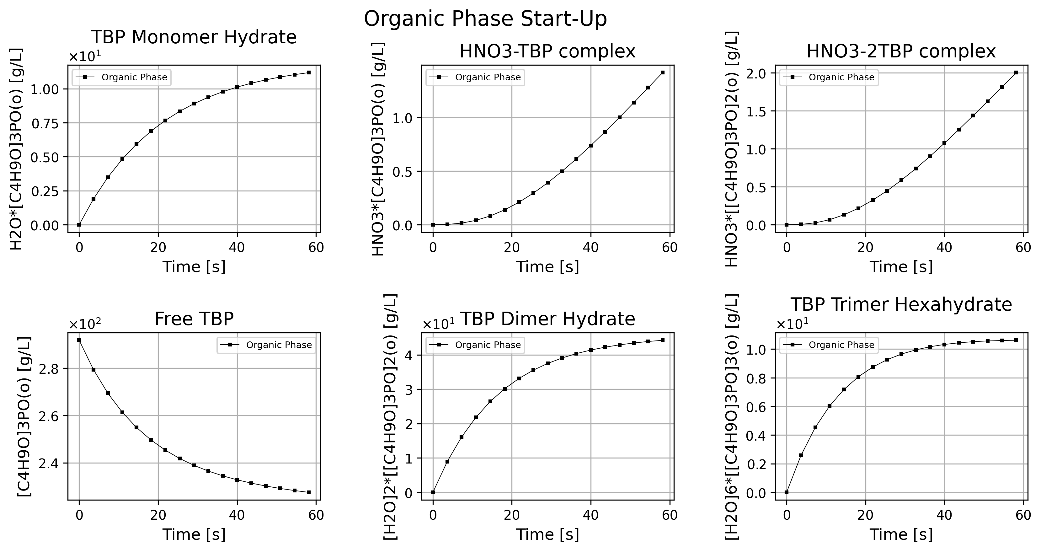
Figure 1: Organic phase species history dashboard at start-up.
Note depletion of free TBP in the organic phase.
Note corresponding complexation of TBP with H2O and HNO3.
Note orders of magnitude of mass concentration in the mixer.
Experimental measurements would be instrumental to help calibrate and validate the model.
'''Organic phase mass density'''
import matplotlib.pyplot as plt

quant = stg.mass_density_history('organic')

quant.plot(title='Organic Phase Mass Density @ %2.1f C Start-Up'%unit.convert_temperature(stg_temperature,
           'K','C'), x_scaling=1/stg.flow_residence_time_avg, x_label=r'Time [$\bar{\tau}$]', y_label=quant.latex_name+r'$-\rho_\text{diluent}$'
           ' ['+quant.unit+']', show=True, figsize=[10,3], error_data=False)

fig_count += 1
print(f'Figure {fig_count}: Organic phase mass density history at start-up.')
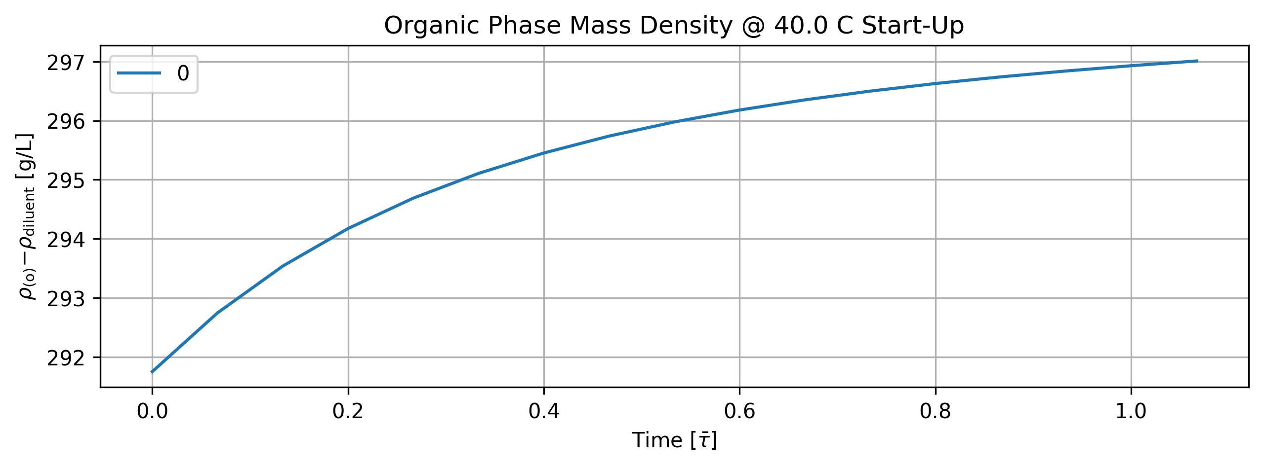
Figure 2: Organic phase mass density history at start-up.
tbl_count += 1
print(f'Table {tbl_count}: Organic phase mass density history at start-up.')
print('Time [s]  Organic Phase Mass Density [g/L]')
print(quant.value[::5].apply(lambda x: round(x,2)))
Table 1: Organic phase mass density history at start-up.
Time [s]  Organic Phase Mass Density [g/L]
0.000000     291.75
18.181818    295.11
36.363636    296.35
54.545455    296.93
Name: Organic Phase Mass Density [g/L]; Time History in [s], dtype: float64
1.5.2. Aqueous Phase Results#
'''Plot aqueous phase'''
# TODO: time axis normalized by phase flow residence time.
stg.aqueous_phase.plot(title='Aqueous Phase Start-Up', legend='Aqueous Phase', nrows=2,ncols=3, show=True, figsize=[12,6])

fig_count += 1
print(f'Figure {fig_count}: Aqueous phase species history dashboard at start-up.')
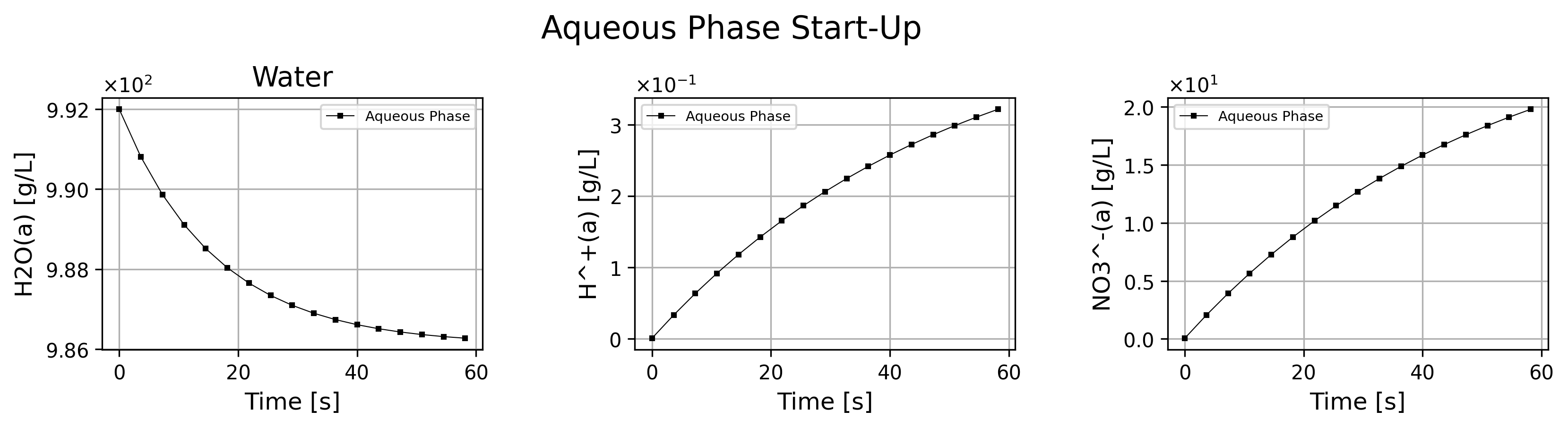
Figure 3: Aqueous phase species history dashboard at start-up.
The inflow feed increases the concentration of all species in the aqueous phase of the mixer.
'''Aqueous phase mass density'''
import matplotlib.pyplot as plt

quant = stg.mass_density_history('aqueous')

quant.plot(title='Aqueous Phase Mass Density @ %2.1f C Start-Up'%unit.convert_temperature(stg_temperature,
           'K','C'), x_scaling=1/stg.flow_residence_time_avg, x_label=r'Time [$\bar{\tau}$]', y_label=quant.latex_name+
           ' ['+quant.unit+']', show=True, figsize=[10,3], error_data=False)

fig_count += 1
print(f'Figure {fig_count}: Aqueous phase mass density history at start-up.')
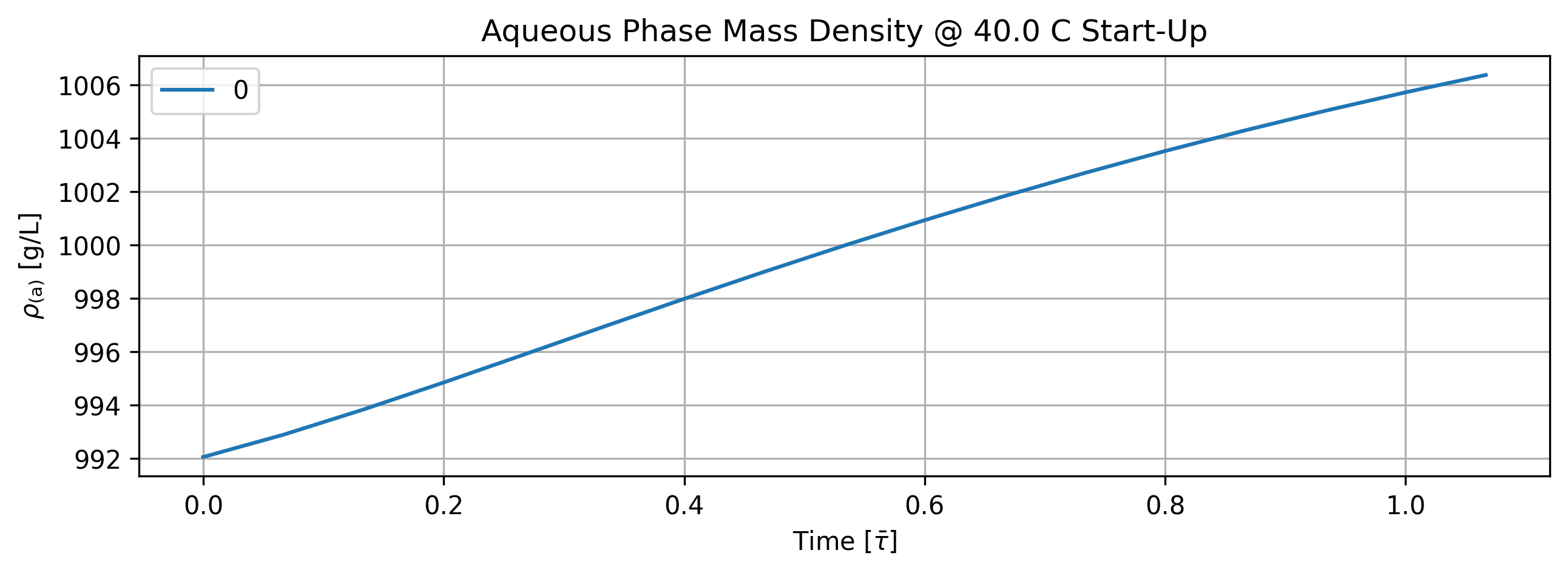
Figure 4: Aqueous phase mass density history at start-up.
tbl_count += 1
print(f'Table {tbl_count}: Aqueous phase mass density history at start-up.')
print('Time [s]  Aqueous Phase Mass Density [g/L]')
print(quant.value[::5].apply(lambda x: round(x,2)))
Table 2: Aqueous phase mass density history at start-up.
Time [s]  Aqueous Phase Mass Density [g/L]
0.000000      992.06
18.181818     996.95
36.363636    1001.84
54.545455    1005.72
Name: Aqueous Phase Mass Density [g/L]; Time History in [s], dtype: float64
1.5.3. Overall Stage Efficiency#
Stage efficiency measures how close to chemical equilibrium the system is as a whole. This is a direct result of the reaction relaxation time which is dependent on the mass transfer coefficients of the system. Much more needs to be investigated in this project with various degrees of theory but these results represent the beginning of a solid development.
'''Stage overall efficiency'''

quant = stg.efficiency_history(mean=True)
quant.plot(title='Stage Efficiency @ %2.1f C Start-Up'%unit.convert_temperature(stg_temperature,
           'K','C'), x_scaling=1/stg.flow_residence_time_avg, x_label=r'Time [$\bar{\tau}$]', y_label=quant.latex_name+
           ' ['+quant.unit+']', show=True, figsize=[10,3], error_data=True)

fig_count += 1
print(f'Figure {fig_count}: Stage efficiency history at start-up.')
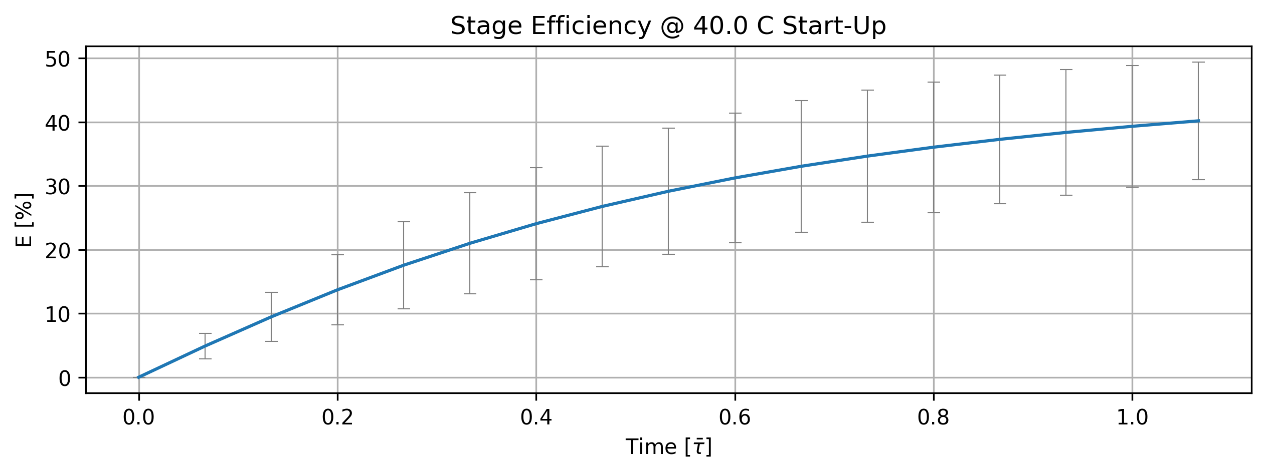
Figure 5: Stage efficiency history at start-up.
tbl_count += 1
print(f'Table {tbl_count}: Stage efficiency history at start-up.')
print('Time [s]  (Stage. Eff., +-std) [%]')
time_name = ''
import pandas as pd
df = (quant.value.apply(pd.Series).mul(1)
       .rename(index=lambda i: round(i/unit.min,2))
       .set_axis(['',''], axis=1).rename_axis(time_name)
       .round(3))
print(df.to_string(max_rows=20, min_rows=20))
Table 3: Stage efficiency history at start-up.
Time [s]  (Stage. Eff., +-std) [%]


0.00   0.000   0.000
0.06   4.876   2.000
0.12   9.457   3.849
0.18  13.695   5.472
0.24  17.550   6.846
0.30  20.987   7.945
0.36  24.059   8.818
0.42  26.768   9.465
0.48  29.147   9.913
0.55  31.231  10.188
0.61  33.053  10.316
0.67  34.649  10.323
0.73  36.047  10.231
0.79  37.277  10.060
0.85  38.362   9.828
0.91  39.324   9.549
0.97  40.179   9.236
'''Individual reaction efficiency'''

quant = stg.efficiency_history()
quant.plot(title='Reaction Efficiency @ %2.1f C Start-Up'%unit.convert_temperature(stg_temperature,
           'K','C'), x_scaling=1/stg.flow_residence_time_avg, x_label=r'Time [$\bar{\tau}$]', y_label=quant.latex_name+
           ' ['+quant.unit+']', legend=stg.rxn_mech.reactions, show=True, figsize=[10,3])

fig_count += 1
print(f'Figure {fig_count}: Reaction efficiency history at start-up.')
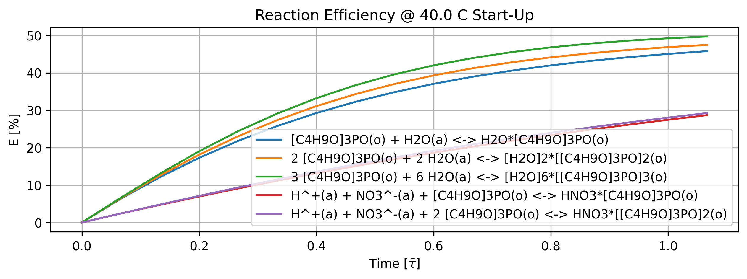
Figure 6: Reaction efficiency history at start-up.
'''Individual reaction efficiency'''

quant = stg.efficiency_history()

tbl_count += 1
print(f'Table {tbl_count}: Reaction efficiency history at start-up.')
print('Time [min]    Rxn Eff. [%]')

col_names = [f'r{i}' for i in range(len(stg.rxn_mech.reactions))]
time_name = ''
df = (quant.value.apply(pd.Series).mul(1)
       .rename(index=lambda i: round(i/unit.min,2))
       .set_axis(col_names, axis=1).rename_axis(time_name)
       .round(3))
print(df.to_string(max_rows=20, min_rows=20))
Table 4: Reaction efficiency history at start-up.
Time [min]    Rxn Eff. [%]
          r0      r1      r2      r3      r4

0.00   0.000   0.000   0.000   0.000   0.000
0.06   6.372   6.506   6.645   2.416   2.443
0.12  12.132  12.583  13.058   4.712   4.802
0.18  17.274  18.119  19.025   6.943   7.114
0.24  21.816  23.063  24.417   9.099   9.356
0.30  25.784  27.351  29.114  11.174  11.512
0.36  29.247  31.098  33.208  13.165  13.576
0.42  32.244  34.304  36.682  15.069  15.541
0.48  34.829  37.023  39.587  16.889  17.409
0.55  37.050  39.311  41.987  18.625  19.180
0.61  38.954  41.224  43.947  20.280  20.860
0.67  40.584  42.817  45.533  21.858  22.451
0.73  41.977  44.136  46.803  23.361  23.960
0.79  43.167  45.226  47.811  24.793  25.390
0.85  44.183  46.123  48.604  26.156  26.746
0.91  45.050  46.860  49.221  27.454  28.032
0.97  45.790  47.464  49.696  28.689  29.253
1.6. Steady-State Simulation#
Pick up from where it left from the past run() and continue to a longer time. This demonstrates how to continue a simulation from where it was interrupted. Note that the state of the system is automatically used as the initial condition for the next run().
end_time += 5 * stg.flow_residence_time_avg
time_step = 5 * stg.flow_residence_time_avg / 15
show_time = (True, 10*time_step)

stg.time_step = time_step
stg.initial_time = stg.end_time
stg.end_time = end_time
stg.show_time = show_time
'''Run system in parallel'''
stg.monitor_mass_flowrates = False
stg.monitor_mass_conservation_residual = False
system.run()
system.close() # Shutdown Cortix
[3365] 2025-11-18 03:04:01,796 - cortix - INFO - Launching Module <solvex.stage.Stage object at 0x7ff1bff43c50>
[14576] 2025-11-18 03:04:03,065 - cortix - INFO - Stg-1::run():time[m]=1.0
[14576] 2025-11-18 03:04:03,226 - cortix - INFO - Stg-1::run():time[m]=4.0
Total mass rate density (mixture volume) residual [g/L-s]= -1.04083e-17
total mass inflow rate [g/min]   = 6.868e+02
total mass outflow rate [g/min]  =  6.868e+02
	 net total mass flow rate [g/min] = -3.344e-02
[14576] 2025-11-18 03:04:03,297 - cortix - INFO - Stg-1::run():time[m]=5.5 (et[s]=0.2)
[3365] 2025-11-18 03:04:03,470 - cortix - INFO - run()::Elapsed wall clock time [s]: 7.18
[3365] 2025-11-18 03:04:03,471 - cortix - INFO - Closed Cortix object.
_____________________________________________________________________________
                           T E R M I N A T I N G
_____________________________________________________________________________
      ...                                        s       .     (TAAG Fraktur)
   xH88"`~ .x8X                                 :8      @88>
 :8888   .f"8888Hf        u.      .u    .      .88      %8P      uL   ..
:8888>  X8L  ^""`   ...ue888b   .d88B :@8c    :888ooo    .     .@88b  @88R
X8888  X888h        888R Y888r ="8888f8888r -*8888888  .@88u  ""Y888k/"*P
88888  !88888.      888R I888>   4888>"88"    8888    888E`    Y888L
88888   %88888      888R I888>   4888> "      8888      888E      8888
88888 `> `8888>     888R I888>   4888>        8888      888E      `888N
`8888L %  ?888   ! u8888cJ888   .d888L .+    .8888Lu=   888E   .u./"888&
 `8888  `-*""   /   "*888*P"    ^"8888*"     ^%888*     888&  d888" Y888*"
   "888.      :"      "Y"          "Y"         "Y"      R888" ` "Y   Y"
     `""***~"`                                           ""
                             https://cortix.org
_____________________________________________________________________________
[3365] 2025-11-18 03:04:03,472 - cortix - INFO - close()::Elapsed wall clock time [s]: 7.18
'''Recover stage'''
stg = system_net.modules[0]
1.6.1. Organic Phase Results#
'''Plot organic phase'''
# TODO: time axis normalized by phase flow residence time.
stg.organic_phase.plot(title='Organic Phase Steady-State', legend='Organic Phase', nrows=2,ncols=3, show=True, figsize=[12,6])

fig_count += 1
print(f'Figure {fig_count}: Organic phase species history dashboard at steady-state.')
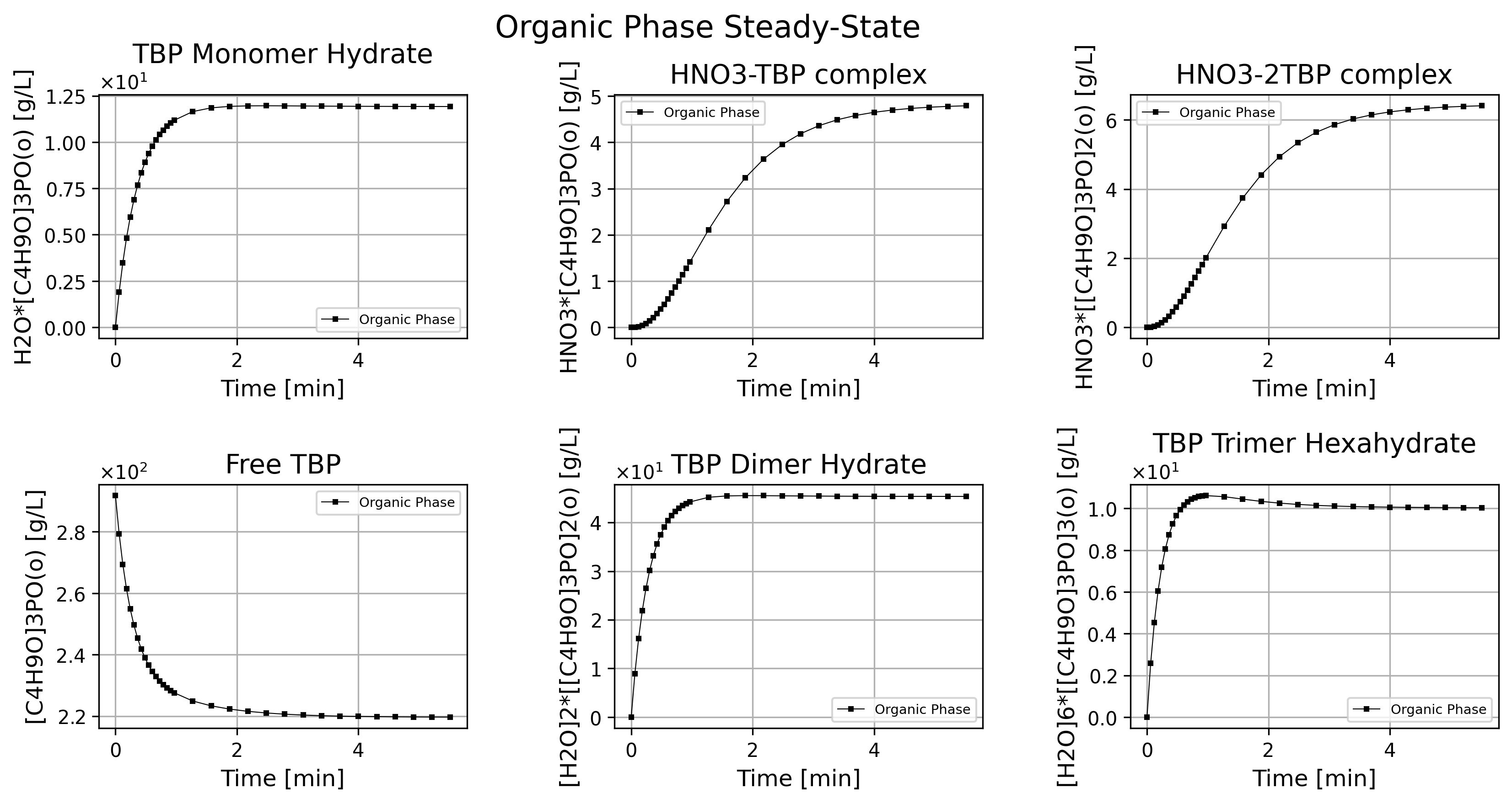
Figure 7: Organic phase species history dashboard at steady-state.
'''Organic phase mass density'''
import matplotlib.pyplot as plt

quant = stg.mass_density_history('organic')

quant.plot(title='Organic Phase Mass Density @ %2.1f C Steady-State'%unit.convert_temperature(stg_temperature,
           'K','C'), x_scaling=1/stg.flow_residence_time_avg, x_label=r'Time [$\bar{\tau}$]', y_label=quant.latex_name+r'$-\rho_\text{diluent}$'
           ' ['+quant.unit+']', show=True, figsize=[10,3], error_data=False)

fig_count += 1
print(f'Figure {fig_count}: Organic phase mass density history at steady-state.')
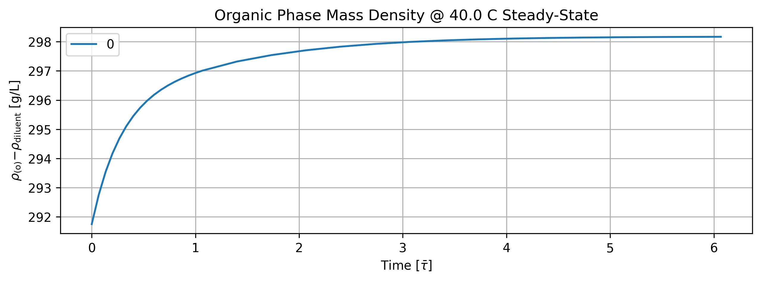
Figure 8: Organic phase mass density history at steady-state.
tbl_count += 1
print(f'Table {tbl_count}: Organic phase mass density history at steady-state.')
print('Time [s]  Organic Phase Mass Density [g/L]')
print(quant.value[::5].apply(lambda x: round(x,2)))
Table 5: Organic phase mass density history at steady-state.
Time [s]  Organic Phase Mass Density [g/L]
0.000000      291.75
18.181818     295.11
36.363636     296.35
54.545455     296.93
130.909091    297.83
221.818182    298.11
312.727273    298.17
Name: Organic Phase Mass Density [g/L]; Time History in [s], dtype: float64
1.6.2. Aqueous Phase Results#
'''Plot aqueous phase'''
# TODO: time axis normalized by phase flow residence time.
stg.aqueous_phase.plot(title='Aqueous Phase Steady-State', legend='Aqueous Phase', nrows=2,ncols=3, show=True, figsize=[12,6])

fig_count += 1
print(f'Figure {fig_count}: Aqueous phase species history dashboard at steady-state.')
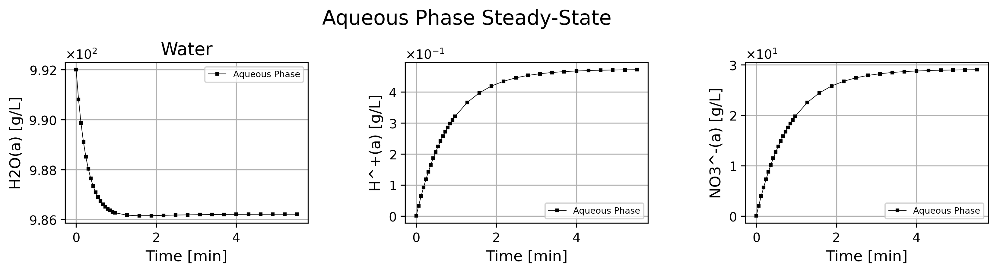
Figure 9: Aqueous phase species history dashboard at steady-state.
'''Aqueous phase mass density'''
import matplotlib.pyplot as plt

quant = stg.mass_density_history('aqueous')

quant.plot(title='Aqueous Phase Mass Density @ %2.1f C Steady-State'%unit.convert_temperature(stg_temperature,
           'K','C'), x_scaling=1/stg.flow_residence_time_avg, x_label=r'Time [$\bar{\tau}$]', y_label=quant.latex_name+
           ' ['+quant.unit+']', show=True, figsize=[10,3], error_data=False)

fig_count += 1
print(f'Figure {fig_count}: Aqueous phase mass density history at Steady-State.')
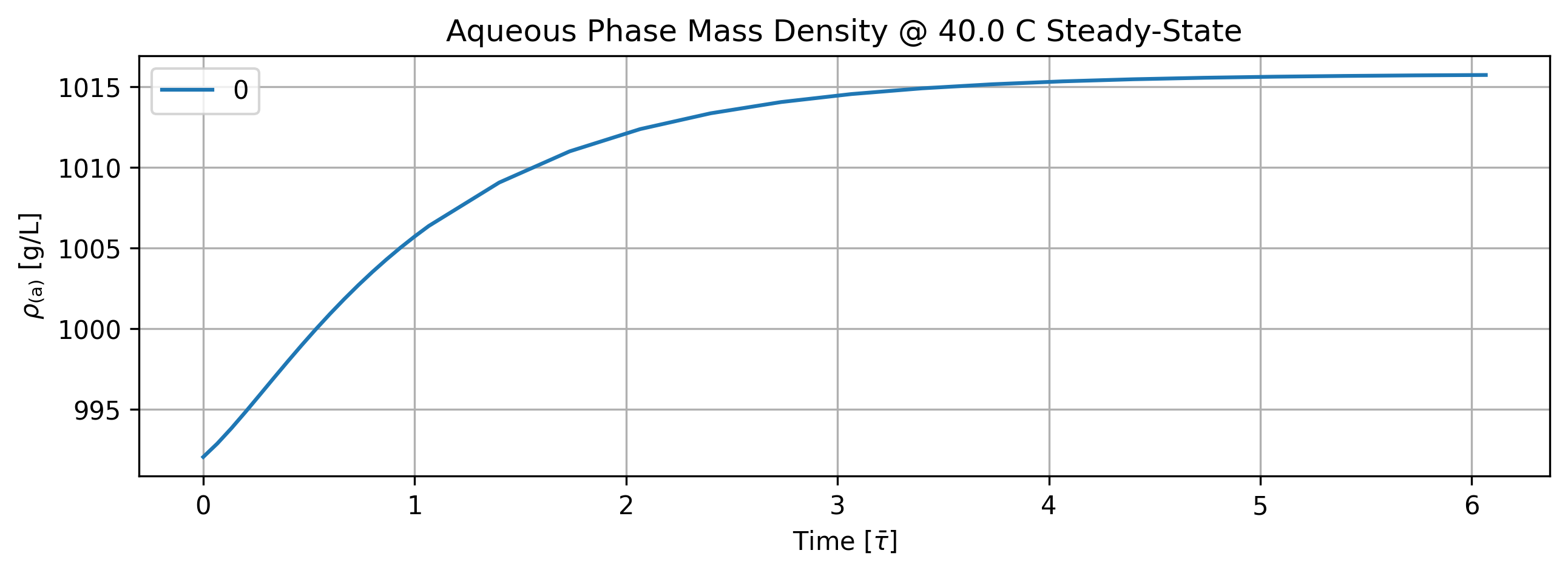
Figure 10: Aqueous phase mass density history at Steady-State.
tbl_count += 1
print(f'Table {tbl_count}: Aqueous phase mass density history at steady-state.')
print('Time [s]  Aqueous Phase Mass Density [g/L]')
print(quant.value[::5].apply(lambda x: round(x,2)))
Table 6: Aqueous phase mass density history at steady-state.
Time [s]  Aqueous Phase Mass Density [g/L]
0.000000       992.06
18.181818      996.95
36.363636     1001.84
54.545455     1005.72
130.909091    1013.36
221.818182    1015.34
312.727273    1015.71
Name: Aqueous Phase Mass Density [g/L]; Time History in [s], dtype: float64
1.6.3. Overall Stage Efficiency#
'''Stage overall efficiency'''

quant = stg.efficiency_history(mean=True)
quant.plot(title='Stage Efficiency @ %2.1f C Steady-State'%unit.convert_temperature(stg_temperature,
           'K','C'), x_scaling=1/stg.flow_residence_time_avg, x_label=r'Time [$\bar{\tau}$]', y_label=quant.latex_name+
           ' ['+quant.unit+']', show=True, figsize=[10,3], error_data=True)

fig_count += 1
print(f'Figure {fig_count}: Stage efficiency history steady-state.')
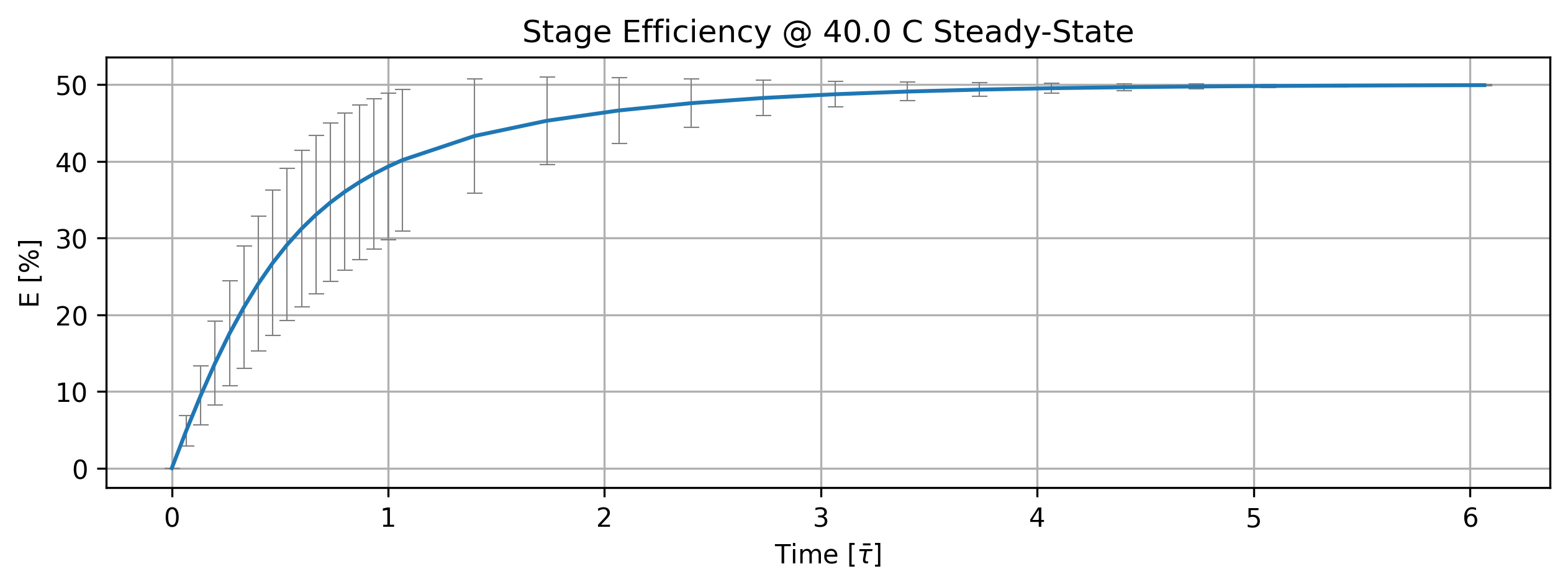
Figure 11: Stage efficiency history steady-state.
tbl_count += 1
print(f'Table {tbl_count}: Stage efficiency history at steady-state.')
print('Time [s]  (Stage. Eff., +-std) [%]')
time_name = ''
import pandas as pd
df = (quant.value.apply(pd.Series).mul(1)
       .rename(index=lambda i: round(i/unit.min,2))
       .set_axis(['',''], axis=1).rename_axis(time_name)
       .round(3))
print(df.to_string(max_rows=20, min_rows=20))
Table 7: Stage efficiency history at steady-state.
Time [s]  (Stage. Eff., +-std) [%]


0.00   0.000   0.000
0.06   4.876   2.000
0.12   9.457   3.849
0.18  13.695   5.472
0.24  17.550   6.846
0.30  20.987   7.945
0.36  24.059   8.818
0.42  26.768   9.465
0.48  29.147   9.913
0.55  31.231  10.188
...      ...     ...
2.79  48.755   1.679
3.09  49.106   1.214
3.39  49.359   0.875
3.70  49.540   0.630
4.00  49.670   0.453
4.30  49.764   0.325
4.61  49.831   0.233
4.91  49.879   0.167
5.21  49.913   0.120
5.52  49.938   0.086
'''Individual reaction efficiency'''

quant = stg.efficiency_history()
quant.plot(title='Reaction Efficiency @ %2.1f C Steady-State'%unit.convert_temperature(stg_temperature,
           'K','C'), x_scaling=1/stg.flow_residence_time_avg, x_label=r'Time [$\bar{\tau}$]', y_label=quant.latex_name+
           ' ['+quant.unit+']', legend=stg.rxn_mech.reactions, show=True, figsize=[10,3])

fig_count += 1
print(f'Figure {fig_count}: Reaction efficiency history at steady-state.')
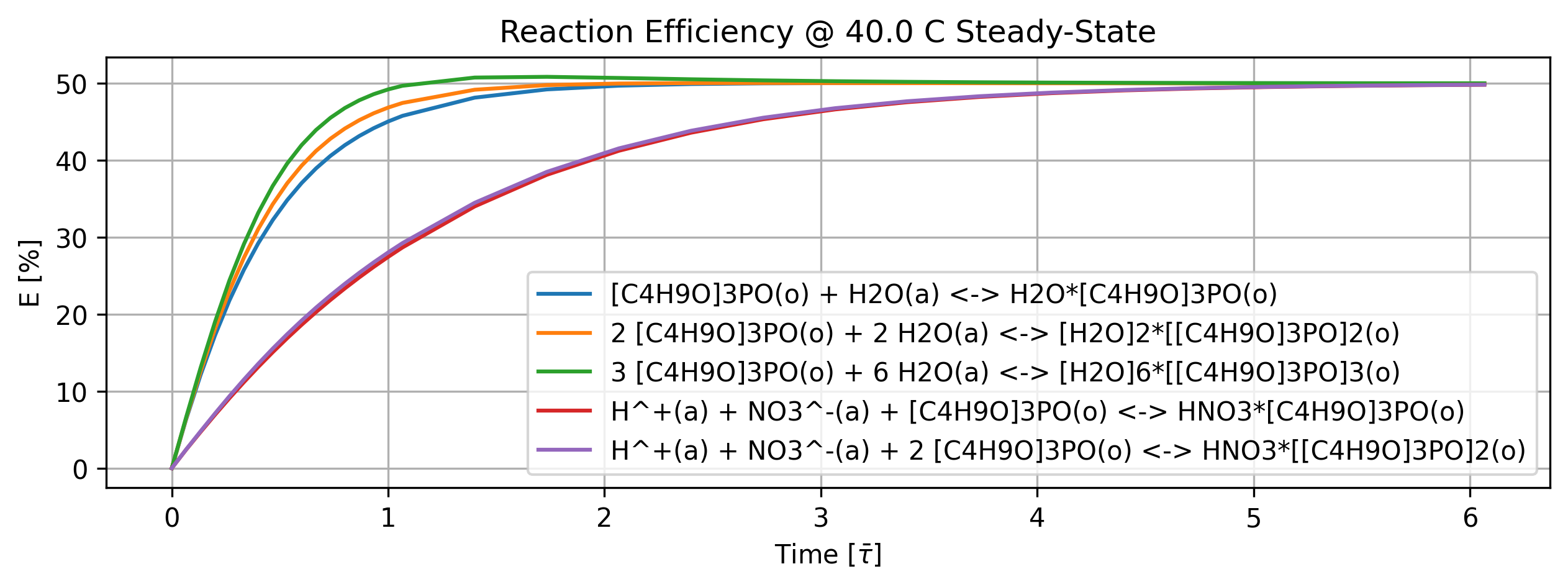
Figure 12: Reaction efficiency history at steady-state.
'''Individual reaction efficiency'''
quant = stg.efficiency_history()
tbl_count += 1
print(f'Table {tbl_count}: Reaction efficiency history at steady-state.')
print('Time [min]    Rxn Eff. [%]')

col_names = [f'r{i}' for i in range(len(stg.rxn_mech.reactions))]
time_name = ''
df = (quant.value.apply(pd.Series).mul(1)
       .rename(index=lambda i: round(i/unit.min,2))
       .set_axis(col_names, axis=1).rename_axis(time_name)
       .round(3))
print(df.to_string(max_rows=20, min_rows=20))
Table 8: Reaction efficiency history at steady-state.
Time [min]    Rxn Eff. [%]
          r0      r1      r2      r3      r4

0.00   0.000   0.000   0.000   0.000   0.000
0.06   6.372   6.506   6.645   2.416   2.443
0.12  12.132  12.583  13.058   4.712   4.802
0.18  17.274  18.119  19.025   6.943   7.114
0.24  21.816  23.063  24.417   9.099   9.356
0.30  25.784  27.351  29.114  11.174  11.512
0.36  29.247  31.098  33.208  13.165  13.576
0.42  32.244  34.304  36.682  15.069  15.541
0.48  34.829  37.023  39.587  16.889  17.409
0.55  37.050  39.311  41.987  18.625  19.180
...      ...     ...     ...     ...     ...
2.79  50.039  50.046  50.284  46.624  46.780
3.09  50.045  50.036  50.205  47.561  47.683
3.39  50.041  50.027  50.147  48.242  48.335
3.70  50.034  50.020  50.106  48.735  48.805
4.00  50.027  50.015  50.076  49.091  49.143
4.30  50.021  50.011  50.055  49.347  49.386
4.61  50.015  50.008  50.039  49.531  49.560
4.91  50.011  50.005  50.028  49.664  49.685
5.21  50.008  50.004  50.020  49.759  49.774
5.52  50.006  50.003  50.014  49.827  49.838
1.7. References#
[1] V. F. de Almeida, Cortix, Network Dynamics Simulation, Cortix Tech, Lowell, MA, USA.