Use-Case 04: TBP-Diluent-H_2O-HNO_3-UO_2^{2+} Mixing

1. Use-Case 04: TBP-Diluent-H\(_2\)O-HNO\(_3\)-UO\(_2^{2+}\) Mixing#

Developer: Valmor F. de Almeida, PhD

Revision date: 02Dec25

1.1. Objectives#

Develop a usecase scenario for water, nitric acid, and uranyl extraction by TBP without a vapor phase.
Test implementation and present results.
Use AI assistants (limited) to help with information and reporting.
- AI requests below may need to be executed multiple times if the result is not satisfactory or incorrect.

'''AI assistance options'''
# Set all to False if you do not have access to OpenAI API and/or AI codes below
cortix_ai = True
stage_ai = True

'''Generate proprietary knowledge database?'''
db_save = False # set this to false if going public (online) with this notebook

'''Other helpers'''
fig_count = 0
tbl_count = 0
markdown_display = True # if False code cell output is type: stream, else: markdown. Use True for in-house conversion to .md

1.2. System#

Single stage mixing of TBP with inert diluent, HNO3 solution with uranyl.

'''Setup the base system'''
from cortix import Cortix
from cortix import Network
from cortix import Units as unit
from cortix import ReactionMechanism
from cortix import Quantity

system = Cortix(use_mpi=False, splash=True) # System top level
system_net = system.network = Network() # Network

if cortix_ai:
    from cortix import CortixAI
    cortix_ai = CortixAI(llm_model='gpt-5-mini', llm_cleverness=0.8)
    cortix_ai.markdown_header_level = '<h3>'
    cortix_ai.n_chunks = 8

if cortix_ai: 
    cortix_ai.explain(markdown_display=markdown_display, save_supporting_info=db_save)

[26493] 2025-12-02 15:11:47,969 - cortix - INFO - Created Cortix object 
_____________________________________________________________________________
                             L A U N C H I N G                               
_____________________________________________________________________________
      ...                                        s       .     (TAAG Fraktur)
   xH88"`~ .x8X                                 :8      @88>
 :8888   .f"8888Hf        u.      .u    .      .88      %8P      uL   ..
:8888>  X8L  ^""`   ...ue888b   .d88B :@8c    :888ooo    .     .@88b  @88R
X8888  X888h        888R Y888r ="8888f8888r -*8888888  .@88u  ""Y888k/"*P
88888  !88888.      888R I888>   4888>"88"    8888    888E`    Y888L
88888   %88888      888R I888>   4888> "      8888      888E      8888
88888 `> `8888>     888R I888>   4888>        8888      888E      `888N
`8888L %  ?888   ! u8888cJ888   .d888L .+    .8888Lu=   888E   .u./"888&
 `8888  `-*""   /   "*888*P"    ^"8888*"     ^%888*     888&  d888" Y888*"
   "888.      :"      "Y"          "Y"         "Y"      R888" ` "Y   Y"
     `""***~"`                                           ""
                             https://cortix.org                              
_____________________________________________________________________________
Cortix AI assistant: working on explanation...

Summary

This snippet imports Cortix framework classes, creates a top-level Cortix system object and an associated Network, and conditionally configures a CortixAI instance if a truthy name cortix_ai is present in the surrounding scope.
Several names are imported but not used in the shown lines (ReactionMechanism, Quantity); Units is aliased to unit.
Two distinct conditional blocks guarded by the same name cortix_ai perform setup and a subsequent call (the final line invokes cortix_ai.explain(…), which is present but will not be described further).

Imports

The code imports Cortix, Network, Units (aliased as unit), ReactionMechanism, and Quantity from the cortix package.
Units is given the local name unit for convenience; ReactionMechanism and Quantity are made available for later use but are not referenced again in this snippet.

System instantiation and network

system = Cortix(use_mpi=False, splash=True)
- Constructs the top-level Cortix system object with two keyword arguments:
  - use_mpi=False: requests a non-MPI (single-process) run.
  - splash=True: requests a startup/banner display (splash) at creation.
system_net = system.network = Network()
- Creates a new Network() instance.
- Assigns that Network object to system.network and also binds it to the local name system_net.
- As a result, the Cortix system now contains an attached Network and the local variable system_net references the same Network object.

Conditional CortixAI setup

First conditional: if cortix_ai:
- The test checks a name cortix_ai in the surrounding scope; that name must be truthy for the block to run.
- Inside the block:
  - from cortix import CortixAI imports the CortixAI class.
  - cortix_ai = CortixAI(llm_model=’gpt-5-mini’, llm_cleverness=0.8) creates a CortixAI instance and assigns it to the name cortix_ai (overwriting whatever value triggered the if).
  - cortix_ai.markdown_header_level = ‘
    ’ sets an attribute to request that the AI produce Markdown using
    header tags.
  - cortix_ai.n_chunks = 8 sets an attribute controlling chunking (number of chunks) for the CortixAI instance.
Second conditional: if cortix_ai:
- Re-evaluates the name cortix_ai; after the previous block this will hold the CortixAI instance when the first block executed.
- The code then calls cortix_ai.explain(markdown_display=markdown_display, save_supporting_info=db_save).
- The call passes two names from the surrounding scope: markdown_display and db_save; these are expected to exist and control output/display and storage behavior respectively.

Notes on names and control flow

The snippet relies on external names (cortix_ai, markdown_display, db_save) being defined before execution. Their values determine whether the CortixAI-related blocks run and what arguments are passed.
The first if block both checks and then overwrites cortix_ai with an instance; so the second if commonly runs immediately afterwards if the first executed.
Several imported symbols (ReactionMechanism, Quantity) are prepared for use later but are unused in the shown lines.

AI Parameters:
+ LLM model (OpenAI) = gpt-5-mini
+ LLM cleverness     = 1.0
+ Total # of tokens  = 3447

'''FYI LLM models info'''
if cortix_ai:
    print(cortix_ai.llm_names_info)

{'gpt-5': 'Full reasoning-intensive tasks', 'gpt-5-mini': 'Balance of speed and capability', 'gpt-5-nano': 'Speed and cost efficiency', 'gpt-4o-mini': 'Fastest at advanced reasoning', 'gpt-4o': 'Great for most tasks', 'gpt-4.1': 'Great for quick coding and analysis', 'gpt-4.1-mini': 'Faster than 4.1 for everyday tasks'}

1.2.1. Stage#

Instantiate a single stage to model and simulate the reactive mixing process.

'''Import Stage'''
from solvex.stage import Stage

'''Create and configure a StageAI object'''
if stage_ai:
    from stage_ai import StageAI
    stage_ai = StageAI(llm_model='gpt-5-mini', llm_cleverness=0.8)
    stage_ai.markdown_header_level = '<h4>'

if stage_ai:
    stage_ai.help('stage', markdown_display=markdown_display, save_supporting_info=db_save)

Stage AI assistant: working on help...

Stage Description

Overview

This report describes the main aspects and structure of the Stage module (a solvent-extraction model) from the provided Stage Knowledge Base. Information about a stage module is needed: stage.

The Stage models three interacting phases (aqueous phase, organic phase, and vapor phase) inside a mixed-volume contactor, integrates reaction mechanisms, and advances the state in time solving mass-balance ODEs for species concentrations.

The original Stage schematics (copied verbatim from the module docstring) follow:

Cortix Module
   This module is a model of a basic solvent extraction stage process.

                          Aqueous    Organic
                         External    Product
                           Feed
                             |          ^
                             |          |
                             |          |
                             V          |
                        |---------------------|
   Vapor/Org inter-stage|                     | Vapor/Aqu inter-stage
   outflow <------------|                     |-----------> outflow
                        |                     |
   Organic inter-stage  |    S O L V E N T    | Aqueous inter-stage
   outflow <------------| E X T R A C T I O N |-----------> outflow
                        |                     |
                        |                     |
   Vapor/Aqu inter-stage|      S T A G E      | Vapor/Org inter-stage
   inflow  ------------>|                     |<----------- inflow
                        |                     |
   Aqueous inter-stage  |                     | Organic inter-stage
   inflow ------------->|                     |<----------- inflow
                        |---------------------|
                             |          ^
                             |          |
                             |          |
                             V          |
                          Aqueous    Organic
                          Product    External
                                       Feed

Phases involved

The Stage explicitly manages three phases: aqueous phase, organic phase, and vapor phase. Each phase is represented with a Phase container that stores species concentration history and time stamps.

Phase names used in the implementation: ‘aqueous’, ‘organic’, ‘vapor’.

Source code structure (high-level)

Module class: Stage(Module)

Initialization sets up:

timing controls (initial_time, end_time, time_step), logging flags, monitoring flags

mixing and per-phase volume fractions derived from volumetric flowrates

flow residence times

three state Phase containers: aqueous_phase, organic_phase, vapor_phase

inflow parameter Phase containers for each phase/interface

placeholders for inflow/outflow species mass-rate numpy vectors

Reaction mechanism support:

add_reaction_mechanism(rxn_mech) populates phases with species and maps global species ids

Time integration and I/O:

run(…) loop: advances time by repeated calls to the internal step method and then calls port communication

step(time): advances state using scipy.integrate.odeint with mbal_rhs_func as RHS

__mbal_rhs_func(u_vec, time, params): ODE right-hand side for mass balances

Utility and history methods: r_vec, g_vec, histories for reaction rates, generation rates, efficiencies, mass densities, and mass-balance residuals

Key class and method signatures (representative, not full bodies)

class Stage(Module)
init(self, mix_vol, vol_flowrates, temperature)
add_reaction_mechanism(self, rxn_mech=None)
run(self, *args)
__step(self, time=0.0)
__mbal_rhs_func(self, u_vec, time, params)
__update_outflow_mass_rates(self, u_vec)
__convert_mass_cc_to_molar_cc(self, u_vec)
__update_state_variables(self, u_vec, time)
r_vec(self, time=None)
g_vec(self, time=None)
rxn_efficiencies(self, time=None)

A brief illustrative snippet (not full implementations):

# Example: important method signatures
class Stage(Module):
    def __init__(self, mix_vol, vol_flowrates, temperature):
        ...
    def add_reaction_mechanism(self, rxn_mech=None):
        ...
    def run(self, *args):
        ...
    def __step(self, time=0.0):
        ...
    def __mbal_rhs_func(self, u_vec, time, params):
        ...

Ports: existence and listing

The Stage exposes interconnection ports to receive/send stream mass-rate data used for composing inflows and outflows. Ports are used inside __call_ports to send/recv stream messages when connected.
Example (single-line Python list of port names):

ports = ['aqu-feed','org-feed','aqu-product','org-product','aqu-inflow','org-inflow','aqu-outflow','org-outflow','vap-aqu-inflow','vap-org-inflow','vap-aqu-outflow','vap-org-outflow']

(here ports are listed but not individually described; the module uses get_port, send, recv and connected_port checks to coordinate communication.)

Usage of ports and call ports methods with time stepping and run()

run(…) implements the top-level time loop:

Update inflow mass rates via __update_mass_inflow_rates() before starting the loop.

For each time step:

Optionally perturb inflow mass rates (stochastic perturbations) via __perturb_mass_inflow_rates().

Call step(time) to integrate one time step (advancing internal state history).

Call call_ports(time) to communicate with connected modules through ports. __call_ports uses:

self.get_port(name).connected_port to decide whether to send/receive

self.send(…) and self.recv(…) for message exchange

Loop ends after end_time.

__call_ports handles both inbound (recv) and outbound (send) interactions depending on connection status; for example, for aqu-inflow the module will recv a (time, mass_inflow_rates) tuple when connected and assert consistency of message time.

What the __step method does (description + source snippet)

Description:

__step assembles the current state vector (mass concentration per species) with __get_state_vector,
sets a short time interval spanning [time, time+time_step], and calls scipy.integrate.odeint with __mbal_rhs_func to integrate the mass-balance ODEs across that interval,
checks integration success, extracts final-state vector, updates mass-conservation diagnostics and optionally prints mass-flowrate monitors, then calls __update_state_variables(u_vec, time) to append the new state to each Phase history container.

Snippet (representative copy from the source; this is the method shown as a snippet):

def __step(self, time=0.0):
    """Stepping Stage in time."""
    u_vec_0 = self.__get_state_vector(time)

    t_interval = np.linspace(time, time+self.time_step, num=2)

    (u_vec_hist, info_dict) = odeint(self.__mbal_rhs_func,
                                     u_vec_0, t_interval,
                                     args=(self.__ode_params,),
                                     full_output=True )

    assert info_dict['message'] == 'Integration successful.'

    u_vec = u_vec_hist[1,:]  # solution vector at final time step

    time += self.time_step

    if self.monitor_mass_conservation_residual or time >= self.end_time:
        self.__check_mass_conservation(u_vec, write=True)
    else:
        self.__check_mass_conservation(u_vec)

    if self.monitor_mass_flowrates or time >= self.end_time:
        (total_mass_inflow_rate, total_mass_outflow_rate) = \
                self.__compute_total_mass_flowrates(u_vec)
        # prints (omitted)

    self.__update_state_variables(u_vec, time)

    return time

The mass balance RHS function: what it is and its signature

Purpose: __mbal_rhs_func is the ODE right-hand-side function that computes time derivatives of the state vector u_vec (mass concentration per species) for the integrator. It assembles source, sink, inflow and outflow contributions and returns dt_u.
Signature (exact):

def __mbal_rhs_func(self, u_vec, time, params):
    """ODE rhs vector function.

    ODE solver sends `u_vec` at time `t` and requests the RHS of the mass balance
    system of equations, that is, `dt_u_vec.`

    `u_vec` is an ordered vector of state variables.
    """

Key steps performed inside __mbal_rhs_func (short description):
- Enforce non-negativity on u_vec (negative values are clamped to zero).
- Call __update_outflow_mass_rates(u_vec) to compute state-derived outflow mass rates per phase.
- Convert mass concentrations into molar concentrations via __convert_mass_cc_to_molar_cc(u_vec).
- Compute species generation rates per mixture volume from the ReactionMechanism: g_vec = rxn_mech.g_vec(…).
- For each phase (aqueous, organic, vapor) compute dt_u entries using: dt_u[gidx] = (inflow_mass_rate - outflow_mass_rate)/mixing_vol + g_vec[gidx] * spc.molar_mass, all scaled by the phase volume fraction phi.
- Return dt_u numpy vector to the integrator.
Units and conventions:
- State vector u_vec holds mass concentration (mass/phase-volume).
- g_vec is returned from the reaction mechanism as molar-generation-rate per mixture volume; the code multiplies g_vec by species molar mass to get mass-generation-rate density.
- The method returns d(mass-concentration)/dt for each species in the global ordering.

Notes on reaction mechanism and species mapping

add_reaction_mechanism(rxn_mech) registers species across phases and sets a global flag (gid) on each species so that u_vec indexing is consistent and global.

The module relies on the ReactionMechanism to provide r_vec and g_vec functions that accept molar-concentration vectors and return reaction rates and species generation rates per mixing-volume.

History and diagnostics utilities

The Stage provides methods to extract time histories (Quantity containers with pandas Series) for:

reaction-rate density history (r_vec_history),

species generation-rate history (g_vec_history),

mass_density_history for a phase,

total mass generation rate density residual history (mass_balance_residual_history),

reaction efficiencies (rxn_efficiencies and efficiency_history) computed from tau-partitioning data in the rxn_mech.

Example minimal usage pattern

Typical sequence:

stg = Stage(mix_vol, vol_flowrates, temperature)

stg.add_reaction_mechanism(rxn_mech)

connect ports as needed (external modules) or provide inflow Phase parameters

stg.run(simulation_args) # run will advance the stage and call ports

Summary

The Stage module is organized around a state vector of species mass concentrations distributed across three phases (aqueous, organic, vapor). It integrates mass-balance ODEs using scipy.integrate.odeint, with a ReactionMechanism providing g and r vectors.
Ports exist to connect inflow/outflow streams and are coordinated inside __call_ports; run() drives the time loop which calls __step() and then __call_ports().
Important methods to inspect for customization: __mbal_rhs_func (RHS signature shown above), __step (time stepping and integration), add_reaction_mechanism (species mapping), and the port interaction logic in __call_ports.

AI Parameters:
+ LLM model (OpenAI) = gpt-5-mini
+ LLM cleverness     = 1.0
+ RAG                = stage.py
+ Total # of tokens  = 18431
Done with help...

1.2.1.1. Configuration#

'''Create Stage and add to base system'''

# Initialization
mix_volume = 1*unit.L
# Aqueous phase
vol_flowrate_aqu = 500*unit.mL/unit.min
# Organic phase
vol_flowrate_org = 600*unit.mL/unit.min
# Vapor phase
vol_flowrate_vap = (0*vol_flowrate_org/100, 0*vol_flowrate_aqu/100) # percentage of (org, aqu)

vol_flowrates = [vol_flowrate_org, vol_flowrate_aqu, vol_flowrate_vap]

stg_temperature = unit.convert_temperature(40, 'C', 'K')

stg = Stage(mix_volume, vol_flowrates, stg_temperature) # Create solvent extraction module

system_net.module(stg) # Add stage module to network

if cortix_ai:
    cortix_ai.explain(markdown_header_level='<h5>', markdown_display=markdown_display, save_supporting_info=db_save)

Cortix AI assistant: working on explanation...

Summary

This snippet constructs a solvent-extraction stage with specified liquid volumes and flowrates, sets its temperature, attaches it to a process network, and conditionally invokes a higher-level explain call.

Parameters and initialization

mix_volume: set to 1 L (unit.L) — the stage hold/mix volume.
vol_flowrate_aqu: aqueous-phase volumetric flow set to 500 mL/min (unit.mL/unit.min).
vol_flowrate_org: organic-phase volumetric flow set to 600 mL/min.
vol_flowrate_vap: a tuple computed as (0 * vol_flowrate_org/100, 0 * vol_flowrate_aqu/100); the comment labels this as “percentage of (org, aqu)”, so the tuple gives vapor-phase percentages for the organic and aqueous streams (both evaluate to zero here).
vol_flowrates: a list grouping [vol_flowrate_org, vol_flowrate_aqu, vol_flowrate_vap].
stg_temperature: temperature converted from 40 °C to kelvin via unit.convert_temperature(40, ‘C’, ‘K’).

Stage creation and network addition

A Stage object is instantiated as stg = Stage(mix_volume, vol_flowrates, stg_temperature). The constructor receives the mix volume, the list of volumetric flow specifications, and the stage temperature.
The created stage is attached to the system network by calling system_net.module(stg), adding that module to the network topology.

Conditional call

The final if-block checks the truthiness of cortix_ai; if present, it invokes cortix_ai.explain with keyword arguments markdown_header_level=’
’, markdown_display=markdown_display, and save_supporting_info=db_save.

AI Parameters:
+ LLM model (OpenAI) = gpt-5-mini
+ LLM cleverness     = 1.0
+ Total # of tokens  = 3408

print('Flow residence time [s]: average = %5.3e'%stg.flow_residence_time_avg)
print('Aqueous volume fraction = %5.3e'%stg.volume_frac_aqu) 
print('Organic volume fraction = %5.3e'%stg.volume_frac_org) 
print('Vapor volume fraction   = %5.3e'%stg.volume_frac_vap) 

Flow residence time [s]: average = 5.455e+01
Aqueous volume fraction = 4.545e-01
Organic volume fraction = 5.455e-01
Vapor volume fraction   = 0.000e+00

'''Draw the Cortix network system'''
system_net.draw(engine='circo', node_shape='folder', ports=True)

../../_images/955457756fd09a8d757eb56107eb2c7ef544d7e34aee257aed96129bbb43b74f.svg

'''For help purposes'''
import solvex.stage

Documentation options:

Live in this notebook run on code cell: help(solvex_ustc.stage)
At ORNL GitLab: source
At UML GitHub: source

# Poor's man help
#help(solvex_ustc.stage)

1.2.2. Reaction Mechanism#

1.2.2.1. Water, nitric acid, and uranyl extraction.#

args_dict = {'water_activity': 1.0}                                                                                                                                                            
file_name='tbp-h2o-hno3-uo22+.txt'                                                                                                                                                      
rxn_mech = ReactionMechanism(file_name=file_name, order_species=True, args_dict=args_dict)           

WARNING: ReactionMechanism: user must implement a H2O*[C4H9O]3PO(o) product partition function with signature <product>(rxn_mech, temperature, spc_molar_cc, arg_dict) function for [C4H9O]3PO(o) + H2O(a) <-> H2O*[C4H9O]3PO(o) 
WARNING: ReactionMechanism: user must implement a [H2O]2*[[C4H9O]3PO]2(o) product partition function with signature <product>(rxn_mech, temperature, spc_molar_cc, arg_dict) function for 2 [C4H9O]3PO(o) + 2 H2O(a) <-> [H2O]2*[[C4H9O]3PO]2(o) 
WARNING: ReactionMechanism: user must implement a [H2O]6*[[C4H9O]3PO]3(o) product partition function with signature <product>(rxn_mech, temperature, spc_molar_cc, arg_dict) function for 3 [C4H9O]3PO(o) + 6 H2O(a) <-> [H2O]6*[[C4H9O]3PO]3(o) 
WARNING: ReactionMechanism: user must implement a HNO3*[C4H9O]3PO(o) product partition function with signature <product>(rxn_mech, temperature, spc_molar_cc, arg_dict) function for H^+(a) + NO3^-(a) + [C4H9O]3PO(o) <-> HNO3*[C4H9O]3PO(o)
WARNING: ReactionMechanism: user must implement a HNO3*[[C4H9O]3PO]2(o) product partition function with signature <product>(rxn_mech, temperature, spc_molar_cc, arg_dict) function for H^+(a) + NO3^-(a) + 2 [C4H9O]3PO(o) <-> HNO3*[[C4H9O]3PO]2(o)
WARNING: ReactionMechanism: user must implement a UO2[NO3]2*[[C4H9O]3PO]2(o) product partition function with signature <product>(rxn_mech, temperature, spc_molar_cc, arg_dict) function for UO2^2+(a) + 2 NO3^-(a) + 2 [C4H9O]3PO(o) <-> UO2[NO3]2*[[C4H9O]3PO]2(o)

#'''User input'''
#rxn_mech.cat_input()

#'''Show Mechanism'''
# Jupyter Book does not render LaTeX through IPython.display(Markdown)
#rxn_mech.md_print()

#'''Species and reactions manual output (copy output and paste into mardown cell)'''
#print(len(rxn_mech.species_names), ' **Species**\n', rxn_mech.latex_species)
#print(len(rxn_mech.reactions), ' **Reactions**\n', rxn_mech.latex_rxn)

11 Species

\[\begin{align*} &{\mathrm{H}_{2}\mathrm{O}}_\mathrm{(a)}, {\mathrm{H}_{2}\mathrm{O}\bullet[\mathrm{C}_{4}\mathrm{H}_{9}\mathrm{O}]_{3}\mathrm{P}\mathrm{O}}_\mathrm{(o)}, {\mathrm{H}\mathrm{N}\mathrm{O}_{3}\bullet[\mathrm{C}_{4}\mathrm{H}_{9}\mathrm{O}]_{3}\mathrm{P}\mathrm{O}}_\mathrm{(o)}, {\mathrm{H}\mathrm{N}\mathrm{O}_{3}\bullet[[\mathrm{C}_{4}\mathrm{H}_{9}\mathrm{O}]_{3}\mathrm{P}\mathrm{O}]_{2}}_{\mathrm{(o)}}, {\mathrm{H}^+}_\mathrm{(a)}, {\mathrm{N}\mathrm{O}_{3}^-}_\mathrm{(a)}, {\mathrm{U}\mathrm{O}_{2}[\mathrm{N}\mathrm{O}_{3}]_{2}\bullet[[\mathrm{C}_{4}\mathrm{H}_{9}\mathrm{O}]_{3}\mathrm{P}\mathrm{O}]_{2}}_{\mathrm{(o)}}, {\mathrm{U}\mathrm{O}_{2}^{2+}}_\mathrm{(a)}, \\ & {[\mathrm{C}_{4}\mathrm{H}_{9}\mathrm{O}]_{3}\mathrm{P}\mathrm{O}}_\mathrm{(o)}, {[\mathrm{H}_{2}\mathrm{O}]_{2}\bullet[[\mathrm{C}_{4}\mathrm{H}_{9}\mathrm{O}]_{3}\mathrm{P}\mathrm{O}]_{2}}_{\mathrm{(o)}}, {[\mathrm{H}_{2}\mathrm{O}]_{6}\bullet[[\mathrm{C}_{4}\mathrm{H}_{9}\mathrm{O}]_{3}\mathrm{P}\mathrm{O}]_{3}}_{\mathrm{(o)}}\end{align*}\]

6 Reactions

\[\begin{align*} {\mathrm{H}_{2}\mathrm{O}}_\mathrm{(a)}\ + \ {[\mathrm{C}_{4}\mathrm{H}_{9}\mathrm{O}]_{3}\mathrm{P}\mathrm{O}}_\mathrm{(o)}\ &\longleftrightarrow \ {\mathrm{H}_{2}\mathrm{O}\bullet[\mathrm{C}_{4}\mathrm{H}_{9}\mathrm{O}]_{3}\mathrm{P}\mathrm{O}}_\mathrm{(o)}\\ 2.0\,{\mathrm{H}_{2}\mathrm{O}}_\mathrm{(a)}\ + \ 2.0\,{[\mathrm{C}_{4}\mathrm{H}_{9}\mathrm{O}]_{3}\mathrm{P}\mathrm{O}}_\mathrm{(o)}\ &\longleftrightarrow \ {[\mathrm{H}_{2}\mathrm{O}]_{2}\bullet[[\mathrm{C}_{4}\mathrm{H}_{9}\mathrm{O}]_{3}\mathrm{P}\mathrm{O}]_{2}}_{\mathrm{(o)}}\\ 6.0\,{\mathrm{H}_{2}\mathrm{O}}_\mathrm{(a)}\ + \ 3.0\,{[\mathrm{C}_{4}\mathrm{H}_{9}\mathrm{O}]_{3}\mathrm{P}\mathrm{O}}_\mathrm{(o)}\ &\longleftrightarrow \ {[\mathrm{H}_{2}\mathrm{O}]_{6}\bullet[[\mathrm{C}_{4}\mathrm{H}_{9}\mathrm{O}]_{3}\mathrm{P}\mathrm{O}]_{3}}_{\mathrm{(o)}}\\ {\mathrm{H}^+}_\mathrm{(a)}\ + \ {\mathrm{N}\mathrm{O}_{3}^-}_\mathrm{(a)}\ + \ {[\mathrm{C}_{4}\mathrm{H}_{9}\mathrm{O}]_{3}\mathrm{P}\mathrm{O}}_\mathrm{(o)}\ &\longleftrightarrow \ {\mathrm{H}\mathrm{N}\mathrm{O}_{3}\bullet[\mathrm{C}_{4}\mathrm{H}_{9}\mathrm{O}]_{3}\mathrm{P}\mathrm{O}}_\mathrm{(o)}\\ {\mathrm{H}^+}_\mathrm{(a)}\ + \ {\mathrm{N}\mathrm{O}_{3}^-}_\mathrm{(a)}\ + \ 2.0\,{[\mathrm{C}_{4}\mathrm{H}_{9}\mathrm{O}]_{3}\mathrm{P}\mathrm{O}}_\mathrm{(o)}\ &\longleftrightarrow \ {\mathrm{H}\mathrm{N}\mathrm{O}_{3}\bullet[[\mathrm{C}_{4}\mathrm{H}_{9}\mathrm{O}]_{3}\mathrm{P}\mathrm{O}]_{2}}_{\mathrm{(o)}}\\ 2.0\,{\mathrm{N}\mathrm{O}_{3}^-}_\mathrm{(a)}\ + \ {\mathrm{U}\mathrm{O}_{2}^{2+}}_\mathrm{(a)}\ + \ 2.0\,{[\mathrm{C}_{4}\mathrm{H}_{9}\mathrm{O}]_{3}\mathrm{P}\mathrm{O}}_\mathrm{(o)}\ &\longleftrightarrow \ {\mathrm{U}\mathrm{O}_{2}[\mathrm{N}\mathrm{O}_{3}]_{2}\bullet[[\mathrm{C}_{4}\mathrm{H}_{9}\mathrm{O}]_{3}\mathrm{P}\mathrm{O}]_{2}}_{\mathrm{(o)}}\\ \end{align*}\]

1.2.2.2. Sanity Check#

'''Data check'''
print('Is mass conserved?', rxn_mech.is_mass_conserved())
rxn_mech.rank_analysis(verbose=True, tol=1e-8)
print('S=\n', rxn_mech.stoic_mtrx)

Is mass conserved? True
# reactions =  6
# species   =  11
rank of S =  6
S is full rank.
S=
 [[-1.  1.  0.  0.  0.  0.  0.  0. -1.  0.  0.]
 [-2.  0.  0.  0.  0.  0.  0.  0. -2.  1.  0.]
 [-6.  0.  0.  0.  0.  0.  0.  0. -3.  0.  1.]
 [ 0.  0.  1.  0. -1. -1.  0.  0. -1.  0.  0.]
 [ 0.  0.  0.  1. -1. -1.  0.  0. -2.  0.  0.]
 [ 0.  0.  0.  0.  0. -2.  1. -1. -2.  0.  0.]]

1.2.2.3. User-Provided Partition Functions#

'''Partition functions involved in the reaction mechanism'''

from solvex.partition_func_local import partition_h2o_tbp_org
from solvex.partition_func_local import partition_2h2o_2tbp_org
from solvex.partition_func_local import partition_6h2o_3tbp_org

# Partition function for H2O*TBP complexation
rxn_mech.data[0]['tau-partition-function'] = partition_h2o_tbp_org

# Partition function for 2H2O*2TBP complexation
rxn_mech.data[1]['tau-partition-function'] = partition_2h2o_2tbp_org

# Partition function for 6H2O*3TBP complexation
rxn_mech.data[2]['tau-partition-function'] = partition_6h2o_3tbp_org

from solvex.partition_func_local import partition_hno3_tbp_org
from solvex.partition_func_local import partition_hno3_2tbp_org

# Partition function for HNO3*TBP complexation
rxn_mech.data[3]['tau-partition-function'] = partition_hno3_tbp_org
  
# Partition function for HNO3*2TBP complexation
rxn_mech.data[4]['tau-partition-function'] = partition_hno3_2tbp_org

from solvex.partition_func_local import partition_uo2no32_2tbp_org

# Partition function for UO2(NO3)2*2TBP complexation
rxn_mech.data[5]['tau-partition-function'] = partition_uo2no32_2tbp_org

if cortix_ai:
    cortix_ai.explain(markdown_header_level='<h5>', markdown_display=markdown_display, save_supporting_info=db_save)

Cortix AI assistant: working on explanation...

Overview

The module-level docstring states the file groups partition functions used in a reaction mechanism. The code imports specific partition-function callables from solvex.partition_func_local and assigns them into entries of rxn_mech.data so each reaction record holds the appropriate partition-function object under the key ‘tau-partition-function’.

Imports

Six partition-function callables are imported (names show the species and stoichiometries they represent):
- partition_h2o_tbp_org
- partition_2h2o_2tbp_org
- partition_6h2o_3tbp_org
- partition_hno3_tbp_org
- partition_hno3_2tbp_org
- partition_uo2no32_2tbp_org

Assignments to rxn_mech.data

The code stores each imported callable into rxn_mech.data at specific indices, using the dictionary key ‘tau-partition-function’:
- rxn_mech.data[0][‘tau-partition-function’] = partition_h2o_tbp_org
- rxn_mech.data[1][‘tau-partition-function’] = partition_2h2o_2tbp_org
- rxn_mech.data[2][‘tau-partition-function’] = partition_6h2o_3tbp_org
- rxn_mech.data[3][‘tau-partition-function’] = partition_hno3_tbp_org
- rxn_mech.data[4][‘tau-partition-function’] = partition_hno3_2tbp_org
- rxn_mech.data[5][‘tau-partition-function’] = partition_uo2no32_2tbp_org

Mapping of indices to chemical complexes

The index-to-function mapping corresponds to these complexes (notations use middle dot for association):
- 0 -> H₂O·TBP complexation
- 1 -> 2 H₂O·2 TBP complexation
- 2 -> 6 H₂O·3 TBP complexation
- 3 -> HNO₃·TBP complexation
- 4 -> HNO₃·2 TBP complexation
- 5 -> UO₂(NO₃)₂·2 TBP complexation

Conditional call at end

A guarded invocation appears:
- if cortix_ai:
  - cortix_ai.explain(markdown_header_level=’
    ’, markdown_display=markdown_display, save_supporting_info=db_save)
This line calls the explain method on the cortix_ai object when cortix_ai evaluates truthy; the call includes the keyword arguments shown (markdown_header_level, markdown_display, save_supporting_info).

Data-structure and intent notes

rxn_mech.data is treated as an indexable collection of per-reaction dictionaries; the code sets one metadata field per reaction to reference a partition-function callable so downstream code can invoke that function when computing tau/partition-related quantities.
The imported names encode which species and how many of each are represented by each partition-function implementation.

AI Parameters:
+ LLM model (OpenAI) = gpt-5-mini
+ LLM cleverness     = 1.0
+ Total # of tokens  = 3882

1.2.2.4. Add Reaction Mechanism to Stage#

stg.add_reaction_mechanism(rxn_mech)

1.2.2.5. Verify Species Groups#

#'''Aqueous phase'''
#str = stg.rxn_mech.md_print('(a)')

#'''Show aqueous phase'''
# Jupyter Book does not render LaTeX through IPython.display(Markdown)
#print(str)

\[\begin{align*} &{\mathrm{H}_{2}\mathrm{O}}_\mathrm{(a)}, \ {\mathrm{H}^+}_\mathrm{(a)}, \ {\mathrm{N}\mathrm{O}_{3}^-}_\mathrm{(a)}, \ {\mathrm{U}\mathrm{O}_{2}^{2+}}_\mathrm{(a)}, \ \end{align*}\]

#'''Organic phase'''
#str = stg.rxn_mech.md_print('(o)', n_species_line=5)

#'''Show organic phase'''
# Jupyter Book does not render LaTeX through IPython.display(Markdown)
#print(str)

\[\begin{align*} &{\mathrm{H}_{2}\mathrm{O}\bullet[\mathrm{C}_{4}\mathrm{H}_{9}\mathrm{O}]_{3}\mathrm{P}\mathrm{O}}_\mathrm{(o)}, \ {\mathrm{H}\mathrm{N}\mathrm{O}_{3}\bullet[\mathrm{C}_{4}\mathrm{H}_{9}\mathrm{O}]_{3}\mathrm{P}\mathrm{O}}_\mathrm{(o)}, \ {\mathrm{H}\mathrm{N}\mathrm{O}_{3}\bullet[[\mathrm{C}_{4}\mathrm{H}_{9}\mathrm{O}]_{3}\mathrm{P}\mathrm{O}]_{2}}_{\mathrm{(o)}}, \ {\mathrm{U}\mathrm{O}_{2}[\mathrm{N}\mathrm{O}_{3}]_{2}\bullet[[\mathrm{C}_{4}\mathrm{H}_{9}\mathrm{O}]_{3}\mathrm{P}\mathrm{O}]_{2}}_{\mathrm{(o)}}, \ {[\mathrm{C}_{4}\mathrm{H}_{9}\mathrm{O}]_{3}\mathrm{P}\mathrm{O}}_\mathrm{(o)}, \\ & {[\mathrm{H}_{2}\mathrm{O}]_{2}\bullet[[\mathrm{C}_{4}\mathrm{H}_{9}\mathrm{O}]_{3}\mathrm{P}\mathrm{O}]_{2}}_{\mathrm{(o)}}, \ {[\mathrm{H}_{2}\mathrm{O}]_{6}\bullet[[\mathrm{C}_{4}\mathrm{H}_{9}\mathrm{O}]_{3}\mathrm{P}\mathrm{O}]_{3}}_{\mathrm{(o)}}, \ \end{align*}\]

1.2.2.6. Mass Transfer Data#

'''Adjust relaxation times for mass transfer'''

rxn_mech.data[0]['tau'] = 1.0e-0 * stg.flow_residence_time_avg
rxn_mech.data[1]['tau'] = 1.0e-0 * stg.flow_residence_time_avg
rxn_mech.data[2]['tau'] = 1.0e-0 * stg.flow_residence_time_avg

rxn_mech.data[3]['tau'] = 1.0e-0 * stg.flow_residence_time_avg
rxn_mech.data[4]['tau'] = 1.0e-0 * stg.flow_residence_time_avg

rxn_mech.data[5]['tau'] = 1.0e-0 * stg.flow_residence_time_avg

if cortix_ai:
    cortix_ai.explain(markdown_header_level='<h5>', markdown_display=markdown_display, save_supporting_info=db_save)

Cortix AI assistant: working on explanation...

Explanation

This snippet assigns relaxation times (tau) for several entries in a reaction-mechanism data structure and then conditionally invokes a method on a cortix_ai object.

The leading triple-quoted string ‘’’Adjust relaxation times for mass transfer’’’ serves as an in-source description/comment for the following code.
rxn_mech.data appears to be an indexable sequence (e.g., list) of dict-like objects; each assignment sets the ‘tau’ key for a specific element: indices 0, 1, 2, 3, 4, and 5 are assigned explicitly.
Each assignment uses 1.0e-0 * stg.flow_residence_time_avg; 1.0e-0 is equal to 1.0, so the multiplier leaves the value unchanged and each ‘tau’ is set equal to stg.flow_residence_time_avg.
The value stg.flow_residence_time_avg is an attribute (on the stg object) that represents the average flow residence time; that value is copied into each specified rxn_mech.data[i][‘tau’].
The assignments are written in three groups (indices 0–2, 3–4, and 5) but together they result in indices 0 through 5 all having the same ‘tau’ value.
The final if-block checks the truthiness of cortix_ai and, if true, calls cortix_ai.explain(…) with three keyword arguments (including markdown_header_level set to ‘
’); no further details about that explain() method are provided here.
In effect, the code standardizes the relaxation time for six reaction-mechanism entries to the stage-average residence time and then optionally triggers the cortix_ai explain invocation.

AI Parameters:
+ LLM model (OpenAI) = gpt-5-mini
+ LLM cleverness     = 1.0
+ Total # of tokens  = 3716

1.2.2.7. Meta Data#

'''Names and info of interest for species'''
  
tbp_org_name = '[C4H9O]3PO(o)'
tbp_org = stg.organic_phase.get_species(tbp_org_name)
tbp_org.info = 'Free TBP'

tbp_monomer_org_name = 'H2O*[C4H9O]3PO(o)'
tbp_monomer_org = stg.organic_phase.get_species(tbp_monomer_org_name)
tbp_monomer_org.info = 'TBP Monomer Hydrate'

tbp_dimer_org_name = '[H2O]2*[[C4H9O]3PO]2(o)'
tbp_dimer_org = stg.organic_phase.get_species(tbp_dimer_org_name)
tbp_dimer_org.info = 'TBP Dimer Hydrate'

tbp_trimer_hexahydrate_org_name = '[H2O]6*[[C4H9O]3PO]3(o)'
tbp_trimer_hexahydrate_org = stg.organic_phase.get_species(tbp_trimer_hexahydrate_org_name)
tbp_trimer_hexahydrate_org.info = 'TBP Trimer Hexahydrate'

uo2no3_2_2tbp_org_name = 'UO2[NO3]2*['+tbp_org_name[:-3]+']2(o)'
uo2no3_2_2tbp_org = stg.organic_phase.get_species(uo2no3_2_2tbp_org_name)
uo2no3_2_2tbp_org.info = r'UO$_2$(NO$_3$)$_2$ * 2TBP'

1.3. Initial Conditions of Mixer#

1.3.1. Organic Phase#

'''Organic phase in the mixer (diluent is inert)'''

vol_frac_tbp_org = 30/100 # free tbp

#TODO: look this up at 40 C # W: TODO: look this up at 40 C
rho_tbp = 972.5 * unit.gram/unit.L # pure liquid TBP
stg.rxn_mech.args_dict['rho-tbp'] = rho_tbp
tbp_mass_cc_org = rho_tbp * vol_frac_tbp_org # per volume of organic phase in the mixture
stg.organic_phase.set_value(tbp_org_name, tbp_mass_cc_org)
print('mass_cc_tbp_org [g/L]  =', tbp_mass_cc_org)
print('molar_cc_tbp_org [M] = %1.5e'%(tbp_mass_cc_org/tbp_org.molar_mass/unit.molar))

mass_cc_tbp_org [g/L]  = 291.75
molar_cc_tbp_org [M] = 1.09551e+00

1.3.2. Aqueous Phase#

'''Aqueous phase in the mixer'''
h2o_aqu = stg.aqueous_phase.get_species('H2O(a)')
h2o_aqu.info = 'Water'
#TODO look this up at 40 C # W: TODO look this up at 40 C
rho_h2o_aqu = 992 * unit.gram/unit.L # per volume of aqueous phase in the mixture
stg.aqueous_phase.set_value('H2O(a)', rho_h2o_aqu)

c_hno3_aqu = 1e-3 * unit.molar # residual
  
h_plus_aqu = stg.aqueous_phase.get_species('H^+(a)')
rho_h_plus_aqu = c_hno3_aqu * h_plus_aqu.molar_mass
stg.aqueous_phase.set_value('H^+(a)', rho_h_plus_aqu)
  
no3_minus_aqu = stg.aqueous_phase.get_species('NO3^-(a)')
rho_no3_minus_aqu = c_hno3_aqu * no3_minus_aqu.molar_mass
stg.aqueous_phase.set_value('NO3^-(a)', rho_no3_minus_aqu)

rho_uo2_2plus_aqu = 0 * unit.gram/unit.L
stg.aqueous_phase.set_value('UO2^2+(a)', rho_uo2_2plus_aqu)

if cortix_ai:
    cortix_ai.explain(markdown_header_level='<h4>', markdown_display=markdown_display, save_supporting_info=db_save)

Cortix AI assistant: working on explanation...

Summary

This Python snippet configures species and their mass concentrations in an aqueous phase object (stg.aqueous_phase) for a mixer context.

Species retrieval and metadata

h2o_aqu = stg.aqueous_phase.get_species(‘H2O(a)’)
h2o_aqu.info = ‘Water’
- Retrieves the aqueous water species object (H₂O(a)) and sets its info/description string to “Water”.
h_plus_aqu = stg.aqueous_phase.get_species(‘H^+(a)’)
- Retrieves the aqueous proton species object (H⁺(a)); the species object is later used for its molar_mass attribute.
no3_minus_aqu = stg.aqueous_phase.get_species(‘NO3^-(a)’)
- Retrieves the aqueous nitrate species object (NO₃⁻(a)).
(Separately) the code references the aqueous uranyl ion species UO₂²⁺(a) when setting a value.

Assigned numerical values and units

rho_h2o_aqu = 992 * unit.gram/unit.L
- Sets a mass density for the aqueous phase water to 992 g·L⁻¹ (comment notes to verify at 40 °C). This value is then assigned to the aqueous phase entry for H₂O(a) via stg.aqueous_phase.set_value(‘H2O(a)’, rho_h2o_aqu).
c_hno3_aqu = 1e-3 * unit.molar
- Defines a residual nitric acid concentration of 1×10⁻³ mol·L⁻¹.
rho_h_plus_aqu = c_hno3_aqu * h_plus_aqu.molar_mass
- Multiplies the molar concentration by the proton species molar mass to produce a mass concentration (mass per L) for H⁺(a). The result is assigned with stg.aqueous_phase.set_value(‘H^+(a)’, rho_h_plus_aqu).
rho_no3_minus_aqu = c_hno3_aqu * no3_minus_aqu.molar_mass
- Analogously computes the NO₃⁻(a) mass concentration from the same molar concentration and assigns it to the aqueous phase.
rho_uo2_2plus_aqu = 0 * unit.gram/unit.L
- Sets the UO₂²⁺(a) mass concentration to 0 g·L⁻¹ and assigns it via stg.aqueous_phase.set_value(‘UO2^2+(a)’, rho_uo2_2plus_aqu).

Conditional call at the end

if cortix_ai: cortix_ai.explain(markdown_header_level=’
’, markdown_display=markdown_display, save_supporting_info=db_save)
- When the variable cortix_ai is truthy, the code invokes its explain method with the given keyword arguments.

AI Parameters:
+ LLM model (OpenAI) = gpt-5-mini
+ LLM cleverness     = 1.0
+ Total # of tokens  = 3991

1.4. Inflow Conditions#

1.4.1. Aqueous Phase#

'''Aqueous phase in the inflow'''
#TODO here the concentration must be larger than in the initial condition in the mixer for lower temp #   W: Line too long (105/100)
# look this up later, 1.01 factor may be incorrect
stg.inflow_aqueous_phase.set_value('H2O(a)', 1.0 * rho_h2o_aqu)

c_hno3_aqu = 0.5 * unit.molar # low acid feed
  
h_plus_aqu = stg.inflow_aqueous_phase.get_species('H^+(a)')
rho_plus_aqu = c_hno3_aqu * h_plus_aqu.molar_mass
stg.inflow_aqueous_phase.set_value('H^+(a)', rho_plus_aqu)
  
no3_minus_aqu = stg.inflow_aqueous_phase.get_species('NO3^-(a)')
rho_no3_minus_aqu = c_hno3_aqu * no3_minus_aqu.molar_mass
stg.inflow_aqueous_phase.set_value('NO3^-(a)', rho_no3_minus_aqu)

rho_uo2_2plus_aqu = 110 * unit.gram/unit.L
stg.inflow_aqueous_phase.set_value('UO2^2+(a)', rho_uo2_2plus_aqu)

if cortix_ai:
    cortix_ai.explain(markdown_header_level='<h4>', markdown_display=markdown_display, save_supporting_info=db_save)

Cortix AI assistant: working on explanation...

Summary

The snippet configures an inflow aqueous phase on an object named stg by assigning mass concentrations for several dissolved species and a solvent, converting from molar concentrations where appropriate.

Line-by-line explanation

The first line is a brief module-level string: “Aqueous phase in the inflow”.
A TODO comment notes a concentration/temperature concern and a suspicious 1.01 factor (comment only; no effect on execution).
stg.inflow_aqueous_phase.set_value(‘H2O(a)’, 1.0 * rho_h2o_aqu)
- Sets the aqueous solvent H₂O(a) to the value 1.0 * rho_h2o_aqu. rho_h2o_aqu is an external variable (presumably a mass concentration or density); the code assigns that scaled value to the inflow phase.
c_hno3_aqu = 0.5 * unit.molar # low acid feed
- Defines a molar concentration of 0.5 mol·L⁻¹ for the nitric-acid-derived H⁺/NO₃⁻ feed (labelled as a “low acid feed”).
h_plus_aqu = stg.inflow_aqueous_phase.get_species(‘H^+(a)’)
- Retrieves the species object corresponding to H⁺(a) from the inflow phase (the returned object is later used for its molar_mass attribute).
rho_plus_aqu = c_hno3_aqu * h_plus_aqu.molar_mass
- Converts the molar concentration c_hno3_aqu (mol·L⁻¹) into a mass concentration (mass·L⁻¹) by multiplying by the species molar mass (mass·mol⁻¹). The resulting unit is mass per volume (e.g., g·L⁻¹) depending on the units on unit.molar and molar_mass.
stg.inflow_aqueous_phase.set_value(‘H^+(a)’, rho_plus_aqu)
- Assigns that computed mass concentration for H⁺(a) into the inflow aqueous phase.
no3_minus_aqu = stg.inflow_aqueous_phase.get_species(‘NO3^-(a)’)
- Retrieves the species object for NO₃⁻(a).
rho_no3_minus_aqu = c_hno3_aqu * no3_minus_aqu.molar_mass
- Converts the same 0.5 mol·L⁻¹ to a mass concentration for NO₃⁻(a) using its molar mass.
stg.inflow_aqueous_phase.set_value(‘NO3^-(a)’, rho_no3_minus_aqu)
- Stores the computed mass concentration for NO₃⁻(a) in the inflow phase.
rho_uo2_2plus_aqu = 110 * unit.gram/unit.L
- Defines a mass concentration of 110 g·L⁻¹ for UO₂²⁺(a).
stg.inflow_aqueous_phase.set_value(‘UO2^2+(a)’, rho_uo2_2plus_aqu)
- Sets UO₂²⁺(a) in the inflow phase to that mass concentration.
if cortix_ai:
- If the name cortix_ai evaluates truthy, the code calls cortix_ai.explain(…). (No explanation of the explain() function is provided.)

Units and conversion notes

c_hno3_aqu is expressed in molar (mol·L⁻¹). Multiplying by a species’ molar_mass (mass·mol⁻¹) yields a mass concentration (mass·L⁻¹), e.g., grams per liter.
The code mixes two patterns for setting concentrations:
- Derived mass concentrations computed from molar inputs (H⁺ and NO₃⁻).
- Direct assignment of a mass concentration for UO₂²⁺.
The exact numeric units depend on the unit objects attached to unit.molar and molar_mass; typical interpretation is mol·L⁻¹ for concentration and g·mol⁻¹ for molar mass, producing g·L⁻¹ for rho_* variables.

AI Parameters:
+ LLM model (OpenAI) = gpt-5-mini
+ LLM cleverness     = 1.0
+ Total # of tokens  = 4055

1.4.2. Organic Phase#

'''Organic phase in the inflow'''
# Set the same mass concentration as the initial condition in the mixer
stg.inflow_organic_phase.set_value(tbp_org_name, tbp_mass_cc_org)

1.5. Start-up Simulation#

Define the start-up simulation period as one flow residence time.

'''Getting ready to run'''

end_time = 1 * stg.flow_residence_time_avg

import numpy as np
ave_tau = np.mean([data['tau'] for data in stg.rxn_mech.data])
time_step = ave_tau / 15
show_time = (True, 10*time_step)

stg.name = 'Stg-1'
stg.save = True
stg.verbose = True

stg.perturb_flowrates = False

stg.time_step = time_step
stg.end_time = end_time
stg.show_time = show_time

'''Run system in parallel'''
stg.monitor_mass_flowrates = False
stg.monitor_mass_conservation_residual = False
stg.mass_bal_rate_dens_res_tol = 1.e-8 * unit.micro*unit.gram/unit.L/unit.second

system.run()
system.close() # Shutdown Cortix

[26493] 2025-12-02 15:16:45,733 - cortix - INFO - Launching Module <solvex.stage.Stage object at 0x7fcf227e34d0>
[27389] 2025-12-02 15:16:47,020 - cortix - INFO - Stg-1::run():time[m]=0.0
[27389] 2025-12-02 15:16:47,259 - cortix - INFO - Stg-1::run():time[m]=0.6
Total mass rate density (mixture volume) residual [g/L-s]= -1.94289e-16
total mass inflow rate [g/min]   = 7.418e+02
total mass outflow rate [g/min]  =  7.160e+02
	 net total mass flow rate [g/min] = -2.580e+01
[27389] 2025-12-02 15:16:47,338 - cortix - INFO - Stg-1::run():time[m]=0.9 (et[s]=0.3)
[26493] 2025-12-02 15:16:47,532 - cortix - INFO - run()::Elapsed wall clock time [s]: 299.56
[26493] 2025-12-02 15:16:47,533 - cortix - INFO - Closed Cortix object.
_____________________________________________________________________________
                           T E R M I N A T I N G                             
_____________________________________________________________________________
      ...                                        s       .     (TAAG Fraktur)
   xH88"`~ .x8X                                 :8      @88>
 :8888   .f"8888Hf        u.      .u    .      .88      %8P      uL   ..
:8888>  X8L  ^""`   ...ue888b   .d88B :@8c    :888ooo    .     .@88b  @88R
X8888  X888h        888R Y888r ="8888f8888r -*8888888  .@88u  ""Y888k/"*P
88888  !88888.      888R I888>   4888>"88"    8888    888E`    Y888L
88888   %88888      888R I888>   4888> "      8888      888E      8888
88888 `> `8888>     888R I888>   4888>        8888      888E      `888N
`8888L %  ?888   ! u8888cJ888   .d888L .+    .8888Lu=   888E   .u./"888&
 `8888  `-*""   /   "*888*P"    ^"8888*"     ^%888*     888&  d888" Y888*"
   "888.      :"      "Y"          "Y"         "Y"      R888" ` "Y   Y"
     `""***~"`                                           ""
                             https://cortix.org                              
_____________________________________________________________________________
[26493] 2025-12-02 15:16:47,534 - cortix - INFO - close()::Elapsed wall clock time [s]: 299.56

'''Recover stage'''
stg = system_net.modules[0]

n_startup = len(stg.organic_phase.time_stamps)

if cortix_ai:
    cortix_ai.explain(markdown_display=markdown_display)

Cortix AI assistant: working on explanation...

Overview

This snippet selects a stage object from a network, counts timestamp entries in that stage’s organic phase, and conditionally invokes a method on a Cortix AI object.

Line-by-line explanation

The first line is a triple-quoted string literal ‘Recover stage’ that serves as an inline documentation string or comment at the top of the snippet.
stg = system_net.modules[0]
- Retrieves the first element (index 0) from the sequence or list system_net.modules and assigns it to the name stg.
n_startup = len(stg.organic_phase.time_stamps)
- Accesses the attribute organic_phase on stg, then the attribute time_stamps on that phase, and computes its length using len(); the resulting integer is stored in n_startup.
if cortix_ai:
- Tests the truthiness of the name cortix_ai; the following indented statement runs only if cortix_ai is truthy (not None, not False, etc.).
- cortix_ai.explain(markdown_display=markdown_display)
  - Calls the explain method on the cortix_ai object, passing the keyword argument markdown_display with the value of the local name markdown_display.

Variables and expected types

system_net.modules: a sequence (e.g., list or tuple) of module-like objects; indexing returns a module instance.
stg: a module-like object expected to have an attribute organic_phase.
stg.organic_phase.time_stamps: an iterable (e.g., list) whose length is meaningful for startup counting.
n_startup: integer equal to the number of entries in time_stamps.
cortix_ai: an object used as a truthy/falsey flag; if truthy it must provide an explain method.
markdown_display: a variable passed as a keyword argument to the method call.

Control flow and side effects

The only control flow is the conditional invocation of cortix_ai.explain; no exceptions are handled in the snippet.
Side effects: assignment to stg and n_startup; a method call may produce external effects depending on the cortix_ai object’s implementation.

AI Parameters:
+ LLM model (OpenAI) = gpt-5-mini
+ LLM cleverness     = 1.0
+ Total # of tokens  = 3210

1.5.1. Organic Phase Results#

'''Plot organic phase'''
# TODO: time axis normalized by phase flow residence time.
stg.organic_phase.plot(title='Organic Phase Start-Up', legend='Organic Phase', nrows=2,ncols=3, show=True, figsize=[12,6])

fig_count += 1
print(f'Figure {fig_count}: Organic phase species history dashboard at start-up.')

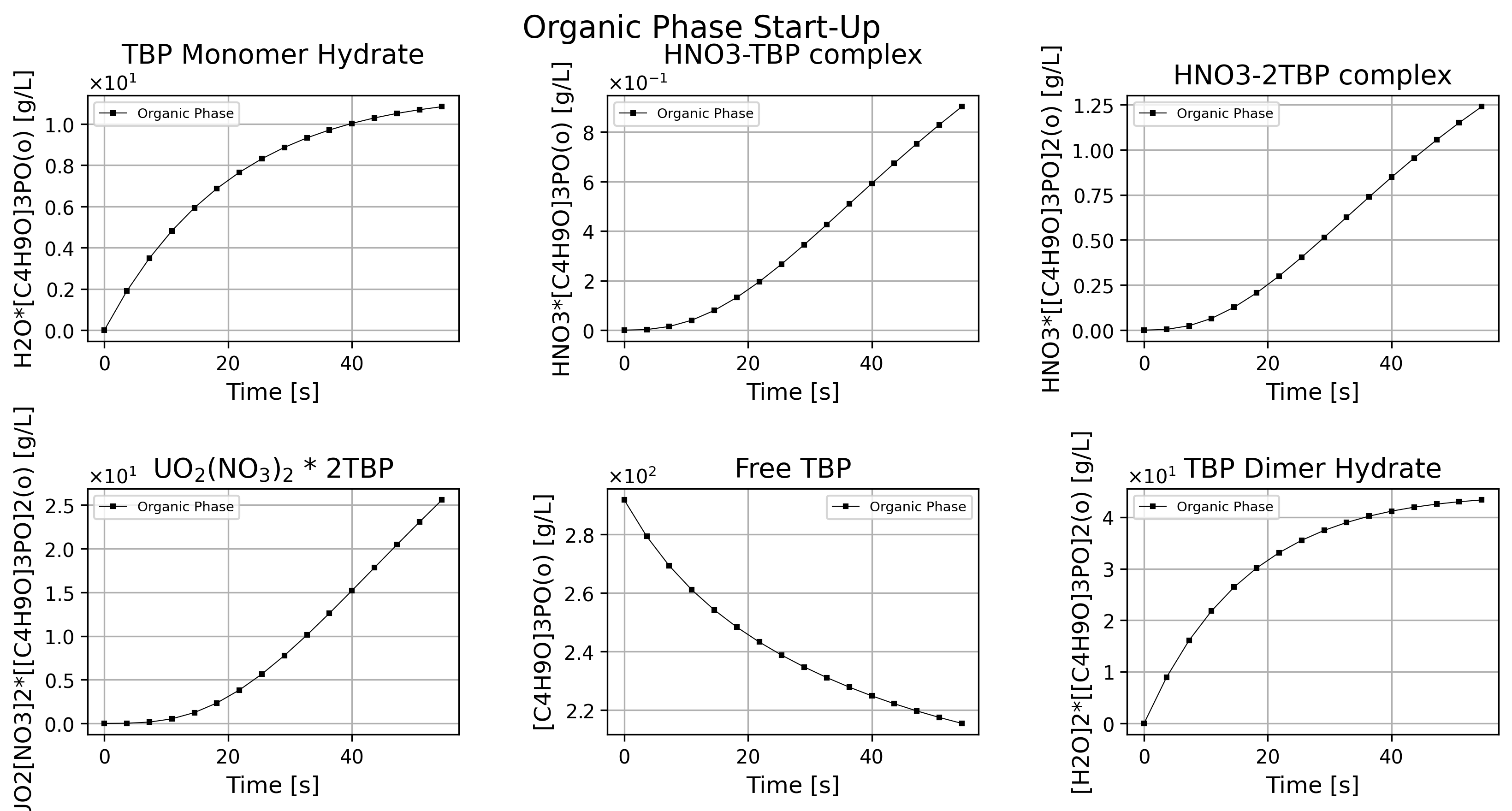
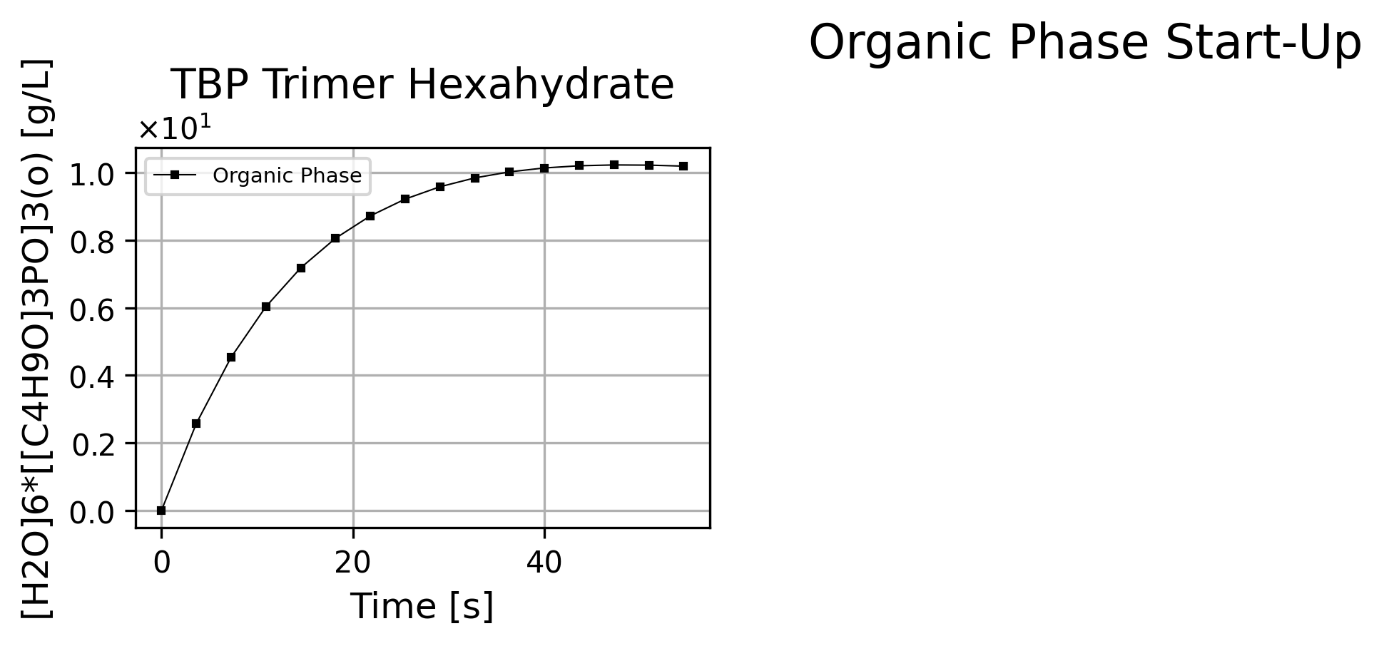
../../_images/d7022fc4fdeaee5e922e7a0215e70d91d75f8cd296d904a9002647d70fb87e33.png

../../_images/70dee50253a116241f29d7f701b3539725e479de8ff360af24b08cc51b0dc504.png

Figure 1: Organic phase species history dashboard at start-up.

Note depletion of free TBP in the organic phase.
Note corresponding complexation of TBP with H2O, HNO3 and uranyl.
Note orders of magnitude of mass concentration in the mixer.
Experimental measurements would be instrumental to help calibrate and validate the model.

if cortix_ai:
    issues = '+ Title your reponse as: Overview of the Organic Phase Data at Start-Up.'
    cortix_ai.explain(phase=stg.organic_phase, issues=issues, markdown_header_level='<h4>', markdown_display=markdown_display, save_supporting_info=db_save)

Cortix AI assistant: working on explanation...

Overview of the Organic Phase Data at Start-Up

Quick summary

The table shows time-resolved concentrations (g/L) in the organic phase during the first 54.5455 s of start-up. Sampling is regular (Δt ≈ 3.63636 s). Free tri-n-butyl phosphate ([C₄H₉O]₃PO(o)) declines steadily while a set of solvated/complexed species (H₂O·[C₄H₉O]₃PO(o), HNO₃·[C₄H₉O]₃PO(o), HNO₃·[[C₄H₉O]₃PO]₂(o), UO₂[NO₃]₂·[[C₄H₉O]₃PO]₂(o), [H₂O]₂·[[C₄H₉O]₃PO]₂(o), [H₂O]₆·[[C₄H₉O]₃PO]₃(o)) increases monotonically.

Sampling cadence: every ~3.63636 s (0, 3.63636, 7.27273, …, 54.5455 s).
Total organic-phase mass (sum of listed species): 291.75 g/L at t = 0 → 307.6004 g/L at t = 54.5455 (net +15.8504 g/L).

Column-by-column analysis (initial → final; units: g/L)

[C₄H₉O]₃PO(o)
- 291.75 → 215.493
- Absolute change: −76.257 g/L (−26.13% of initial)
- Average rate: −1.399 g·L⁻¹·s⁻¹
H₂O·[C₄H₉O]₃PO(o)
- 0 → 10.8402
- Absolute change: +10.8402 g/L
- Average rate: +0.199 g·L⁻¹·s⁻¹
HNO₃·[C₄H₉O]₃PO(o)
- 0 → 0.902605
- Absolute change: +0.902605 g/L
- Average rate: +0.0166 g·L⁻¹·s⁻¹
HNO₃·[[C₄H₉O]₃PO]₂(o)
- 0 → 1.23869
- Absolute change: +1.23869 g/L
- Average rate: +0.0227 g·L⁻¹·s⁻¹
UO₂[NO₃]₂·[[C₄H₉O]₃PO]₂(o)
- 0 → 25.5828
- Absolute change: +25.5828 g/L
- Average rate: +0.469 g·L⁻¹·s⁻¹
[H₂O]₂·[[C₄H₉O]₃PO]₂(o)
- 0 → 43.3519
- Absolute change: +43.3519 g/L
- Average rate: +0.794 g·L⁻¹·s⁻¹
[H₂O]₆·[[C₄H₉O]₃PO]₃(o)
- 0 → 10.1912
- Absolute change: +10.1912 g/L
- Average rate: +0.187 g·L⁻¹·s⁻¹

Comparative observations and shares (at t = 54.5455 s)

Largest absolute increases: [H₂O]₂·[[C₄H₉O]₃PO]₂(o) (+43.35 g/L) and UO₂[NO₃]₂·[[C₄H₉O]₃PO]₂(o) (+25.58 g/L).
Free [C₄H₉O]₃PO remains the major single component but has declined to ~70.1% of the total listed organic-phase concentration at the last time point.
Relative fractions of total organic-phase concentration at t = 54.5455 s (total ≈ 307.60 g/L):
- [C₄H₉O]₃PO(o): ~70.1%
- [H₂O]₂·[[C₄H₉O]₃PO]₂(o): ~14.1%
- UO₂[NO₃]₂·[[C₄H₉O]₃PO]₂(o): ~8.3%
- H₂O·[C₄H₉O]₃PO(o): ~3.5%
- [H₂O]₆·[[C₄H₉O]₃PO]₃(o): ~3.3%
- HNO₃-containing complexes combined: ~0.7%

Notes on trends and interpretation of the data

All complexed/solvated species increase monotonically with time; none show transient maxima or decreases within the sampled interval.
The free ligand pool decreases steadily, consistent with ligand binding/solvation and uptake of metal nitrate and water into the organic phase.
The UO₂-containing complex accrues substantially faster than the simple HNO₃ adducts, indicating significant metal transfer into the organic phase relative to nitric acid-only complexation (within this time window).
The total listed organic concentration rises modestly (+15.85 g/L), indicating net uptake from the aqueous phase (water, HNO₃, UO₂ species) into the organic phase during start-up.

Key takeaways

Start-up induces rapid complexation and solvation of [C₄H₉O]₃PO(o): the ligand pool falls ~26% over ~54.5 s while multiple complexes form.
Water-associated complexes ([H₂O]₂·… and H₂O·…) account for the largest increases collectively.
UO₂ transfer into the organic phase is substantial and represents a significant share (~8.3%) of the organic-phase mass at 54.5455 s.

AI Parameters:
+ LLM model (OpenAI) = gpt-5-mini
+ LLM cleverness     = 1.0
+ Total # of tokens  = 8023

'''Organic phase mass density'''
import matplotlib.pyplot as plt

quant = stg.mass_density_history('organic')

quant.plot(title='Organic Phase Mass Density @ %2.1f C Start-Up'%unit.convert_temperature(stg_temperature,
           'K','C'), x_scaling=1/stg.flow_residence_time_avg, x_label=r'Time [$\bar{\tau}$]', y_label=quant.latex_name+r'$-\rho_\text{diluent}$'+
           ' ['+quant.unit+']', show=True, figsize=[10,3], error_data=False)

fig_count += 1
print(f'Figure {fig_count}: Organic phase mass density history at start-up.')

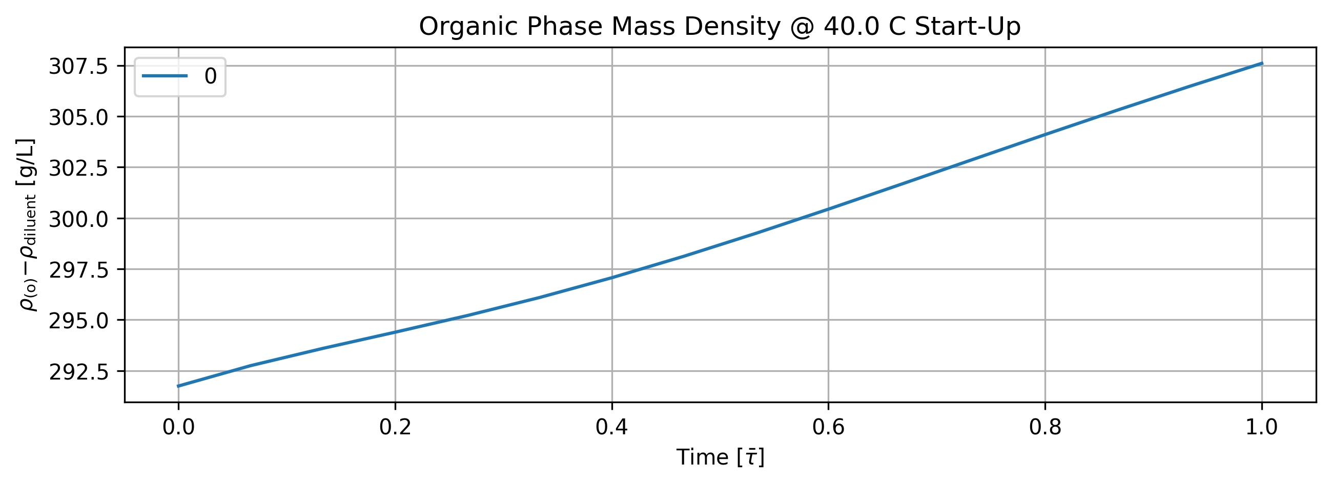
../../_images/5b62c025a7a6017a432a9b9efc686385bd3a01b0b07d30b73270b4457bfcfe67.png

Figure 2: Organic phase mass density history at start-up.

tbl_count += 1
print(f'Table {tbl_count}: Organic phase mass density history at start-up.')
print('Time [s]  Organic Phase Mass Density [g/L]')
print(quant.value[::5].apply(lambda x: round(x,2)))

Table 1: Organic phase mass density history at start-up.
Time [s]  Organic Phase Mass Density [g/L]
0.000000     291.75
18.181818    296.10
36.363636    301.65
54.545455    307.60
Name: Organic Phase Mass Density [g/L]; Time History in [s], dtype: float64

1.5.2. Aqueous Phase Results#

'''Plot aqueous phase'''
# TODO: time axis normalized by phase flow residence time.
stg.aqueous_phase.plot(title='Aqueous Phase Start-Up', legend='Aqueous Phase', nrows=2,ncols=3, show=True, figsize=[12,6])

fig_count += 1
print(f'Figure {fig_count}: Aqueous phase species history dashboard at start-up.')

../../_images/448727e80ac7aa51e36eb65cd7864a450ab0f328f3b3bfb03bc44fa18ebf2641.png

Figure 3: Aqueous phase species history dashboard at start-up.

if cortix_ai:
    issues = '+ Title your reponse as: Overview of the Aqueous Phase Data at Start-Up.\n'
    cortix_ai.explain(phase=stg.aqueous_phase, issues=issues, markdown_header_level='<h4>', markdown_display=markdown_display, save_supporting_info=db_save)

Cortix AI assistant: working on explanation...

Overview of the Aqueous Phase Data at Start-Up.

Overall observations

The table records concentrations (g/L) at 16 time points from 0 to 54.5455 s for H₂O(a), H⁺(a), NO₃⁻(a) and UO₂²⁺(a).
All solute concentrations (H⁺, NO₃⁻, UO₂²⁺) increase monotonically; the solvent H₂O(a) decreases monotonically.
Changes are continuous and non-linear: per-interval increments for solutes diminish with time (decelerating growth), consistent with an approach toward a slower accumulation rate or a limiting process.

Trends by species

H₂O(a):
- Decreases from 992 g/L to 986.422 g/L (Δ = −5.578 g/L, −0.563%).
- Average rate ≈ −0.102 g·L⁻¹·s⁻¹ over the 54.5455 s period.
- Per-interval losses shrink slightly with time (rate of decrease slows).
H⁺(a):
- Rises from 0.00100739 g/L to 0.31294 g/L (Δ ≈ +0.31193 g/L).
- Average rate ≈ +0.00572 g·L⁻¹·s⁻¹.
- Fold increase ≈ 310× relative to initial concentration.
- Increment per time step decreases steadily (concave-up temporal profile in concentration vs time).
NO₃⁻(a):
- Rises from 0.0620055 g/L to 15.1589 g/L (Δ ≈ +15.0969 g/L).
- Average rate ≈ +0.2768 g·L⁻¹·s⁻¹.
- Fold increase ≈ 245×.
- Per-interval increases decline with time, indicating decelerating accumulation.
UO₂²⁺(a):
- Rises from 0 to 60.5577 g/L (Δ = +60.5577 g/L).
- Average rate ≈ +1.1101 g·L⁻¹·s⁻¹.
- Largest absolute increase of the four species.
- Per-interval gains are large initially and then progressively smaller, showing a strong deceleration in accumulation.

Quantitative comparisons and mass context

Absolute accumulation ranking (final − initial): UO₂²⁺ (≈60.56 g/L) > NO₃⁻ (≈15.10 g/L) > H⁺ (≈0.3129 g/L) > H₂O (decrease ≈5.58 g/L).
Net increase in dissolved solute mass ≈ 75.967 g/L (initial ≈0.0630 g/L → final ≈76.0306 g/L), while H₂O decreased by only ≈5.58 g/L. This indicates a large addition or production of solute mass relative to solvent loss over the sampled period.
Relative rates: UO₂²⁺ accumulates an order of magnitude faster (by absolute g/L·s) than NO₃⁻, which in turn accumulates faster than H⁺; H₂O shows a small negative rate.

Summary

The dataset shows monotonic, decelerating accumulation of solutes (H⁺, NO₃⁻, UO₂²⁺) and a small, steady loss of H₂O(a) over 0–54.5455 s.
UO₂²⁺ dominates the absolute concentration changes; NO₃⁻ is the second major contributor; H⁺ changes are quantitatively small but large in fold-change terms from a very low baseline.
The pattern of diminishing per-step increases across solutes suggests the system is moving toward a slower dynamic regime (e.g., approaching a limit, saturation, or reduced driving force) during the sampled start-up interval.

AI Parameters:
+ LLM model (OpenAI) = gpt-5-mini
+ LLM cleverness     = 1.0
+ Total # of tokens  = 5895

The inflow feed increases the concentration of all species in the aqueous phase of the mixer.

'''Aqueous phase mass density'''
import matplotlib.pyplot as plt

quant = stg.mass_density_history('aqueous')

quant.plot(title='Aqueous Phase Mass Density @ %2.1f C Start-Up'%unit.convert_temperature(stg_temperature,
           'K','C'), x_scaling=1/stg.flow_residence_time_avg, x_label=r'Time [$\bar{\tau}$]', y_label=quant.latex_name+
           ' ['+quant.unit+']', show=True, figsize=[10,3], error_data=False)

fig_count += 1
print(f'Figure {fig_count}: Aqueous phase mass density history at start-up.')

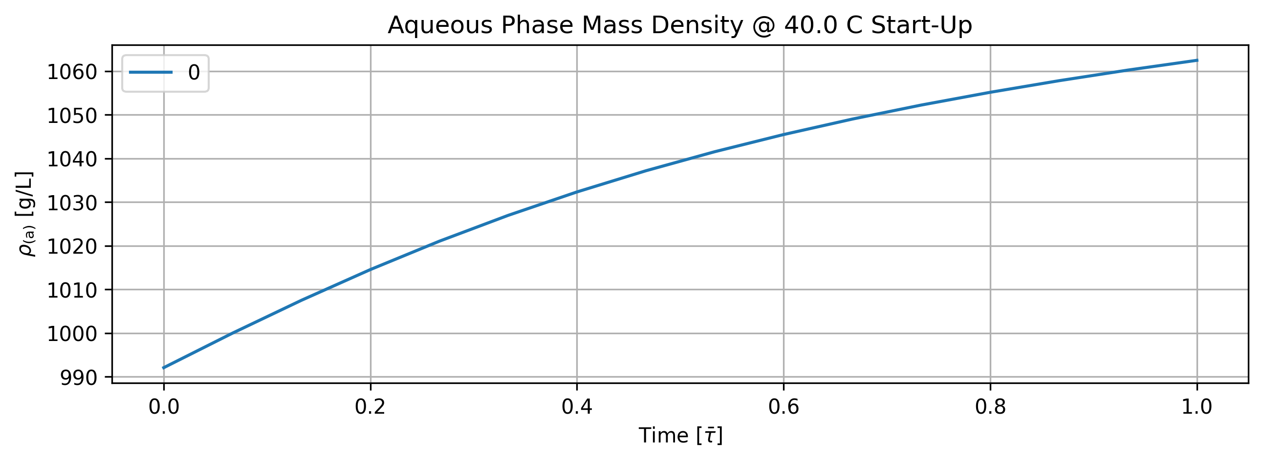
../../_images/0ffa914266a85537bea60baa097fea4c37815ab5a7be0911da2860c74710488c.png

Figure 4: Aqueous phase mass density history at start-up.

tbl_count += 1
print(f'Table {tbl_count}: Aqueous phase mass density history at start-up.')
print('Time [s]  Aqueous Phase Mass Density [g/L]')
print(quant.value[::5].apply(lambda x: round(x,2)))

Table 2: Aqueous phase mass density history at start-up.
Time [s]  Aqueous Phase Mass Density [g/L]
0.000000      992.06
18.181818    1026.94
36.363636    1049.00
54.545455    1062.45
Name: Aqueous Phase Mass Density [g/L]; Time History in [s], dtype: float64

1.5.3. Overall Stage Efficiency#

Stage efficiency measures how close to chemical equilibrium the system is as a whole. This is a direct result of the reaction relaxation time which is dependent on the mass transfer coefficients of the system. Much more needs to be investigated in this project with various degrees of theory but these results represent the beginning of a solid development.

'''Stage overall efficiency'''

quant = stg.efficiency_history(mean=True)
quant.plot(title='Stage Efficiency @ %2.1f C Start-Up'%unit.convert_temperature(stg_temperature,
           'K','C'), x_scaling=1/stg.flow_residence_time_avg, x_label=r'Time [$\bar{\tau}$]', y_label=quant.latex_name+
           ' ['+quant.unit+']', show=True, figsize=[10,3], error_data=True)

fig_count += 1
print(f'Figure {fig_count}: Stage efficiency history at start-up.')

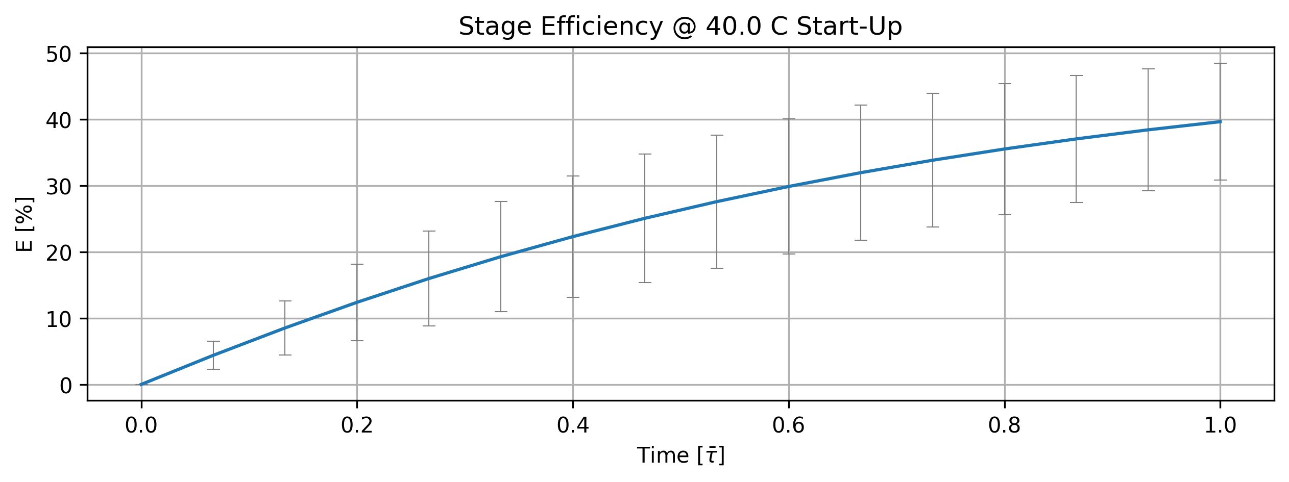
../../_images/e02ded53dd6e7757ca15a7642e685b848e8cca07d5205f945a947479590ec6b7.png

Figure 5: Stage efficiency history at start-up.

tbl_count += 1
print(f'Table {tbl_count}: Stage efficiency history at start-up.')
print('Time [s]  (Stage. Eff., +-std) [%]')
time_name = ''
import pandas as pd
df = (quant.value.apply(pd.Series).mul(1)
       .rename(index=lambda i: round(i/unit.min,2))
       .set_axis(['',''], axis=1).rename_axis(time_name)
       .round(3))
print(df.to_string(max_rows=20, min_rows=20))

Table 3: Stage efficiency history at start-up.
Time [s]  (Stage. Eff., +-std) [%]
                    
                    
00   0.000   0.000
06   4.387   2.129
12   8.530   4.088
18  12.400   5.777
24  15.990   7.185
30  19.291   8.301
36  22.316   9.136
42  25.078   9.715
48  27.596  10.069
55  29.887  10.230
61  31.966  10.234
67  33.847  10.109
73  35.545   9.886
79  37.073   9.589
85  38.444   9.238
91  39.671   8.850

if cortix_ai:
    issues = '+ Title your reponse as: Overview of the Stage Efficiency Data at Start-Up.'
    cortix_ai.explain(quant=quant, issues=issues, markdown_header_level='<h4>', markdown_display=markdown_display, save_supporting_info=db_save, print_prompt=False)

Cortix AI assistant: working on explanation...

Overview of the Stage Efficiency Data at Start-Up

Summary

Dataset: 8 measurements (rows 0–7). Columns are row index, time [s], mean stage efficiency [%], and standard deviation [%].
Time range: 0 s to 50.9091 s, sampled every 7.27273 s (uniform spacing).
Units: dependent quantity is efficiency in percent (%). Table reports mean ± standard deviation (columns labeled “0” = mean, “1” = standard deviation).
Broad trend: mean efficiency rises monotonically from 0% to 38.4441% over the measured interval; spread (std) increases early and then plateaus.

Quantitative metrics (computed from the table)

Mean of the mean efficiencies: 22.55%.
Median of the mean efficiencies: 24.96%.
Minimum mean efficiency: 0% at 0 s. Maximum mean efficiency: 38.4441% at 50.9091 s.
Mean of the reported standard deviations: 7.48%.
Median of the standard deviations: 9.19%.
Maximum absolute standard deviation: 10.2335% at 36.3636 s; minimum 0% at 0 s.
Overall average growth rate (0 -> 50.9091 s): ≈ 0.755 % per s.
Representative instantaneous growth rates:
- 0 -> 7.27273 s: ≈ 1.17 %/s
- 36.3636 -> 43.6364 s: ≈ 0.49 %/s
- 43.6364 -> 50.9091 s: ≈ 0.40 %/s
Coefficient of variation (std / mean) trend:
- 7.2727 s: 47.9%
- 14.5455 s: 44.9%
- 21.8182 s: 41.0%
- 29.0909 s: 36.5%
- 36.3636 s: 32.0%
- 43.6364 s: 27.8%
- 50.9091 s: 24.0%

Observations and interpretation

The mean efficiency increases steadily during start-up but with a decreasing growth rate: early increases are faster, later increases slow, indicating approach toward a plateau or steady operating regime.
Absolute variability (std) rises from start, peaks near 36.36 s (10.2335%), then slightly declines toward the end; relative variability (coefficient of variation) falls continuously, indicating measurements become more consistent in relative terms as efficiency rises.
Uniform time spacing supports straightforward temporal trend interpretation; row index is simply the measurement index (not an additional variable).
Key numbers for reporting: final mean = 38.4441% (at 50.9091 s), peak std = 10.2335% (at 36.3636 s), and the decreasing CV to ~24% at the last time point.

AI Parameters:
+ LLM model (OpenAI) = gpt-5-mini
+ LLM cleverness     = 1.0
+ Total # of tokens  = 5324

'''Individual reaction efficiency'''

quant = stg.efficiency_history()
quant.plot(title='Reaction Efficiency @ %2.1f C Start-Up'%unit.convert_temperature(stg_temperature,
           'K','C'), x_scaling=1/stg.flow_residence_time_avg, x_label=r'Time [$\bar{\tau}$]', y_label=quant.latex_name+
           ' ['+quant.unit+']', legend=stg.rxn_mech.reactions, show=True, figsize=[10,3])

fig_count += 1
print(f'Figure {fig_count}: Reaction efficiency history at start-up.')

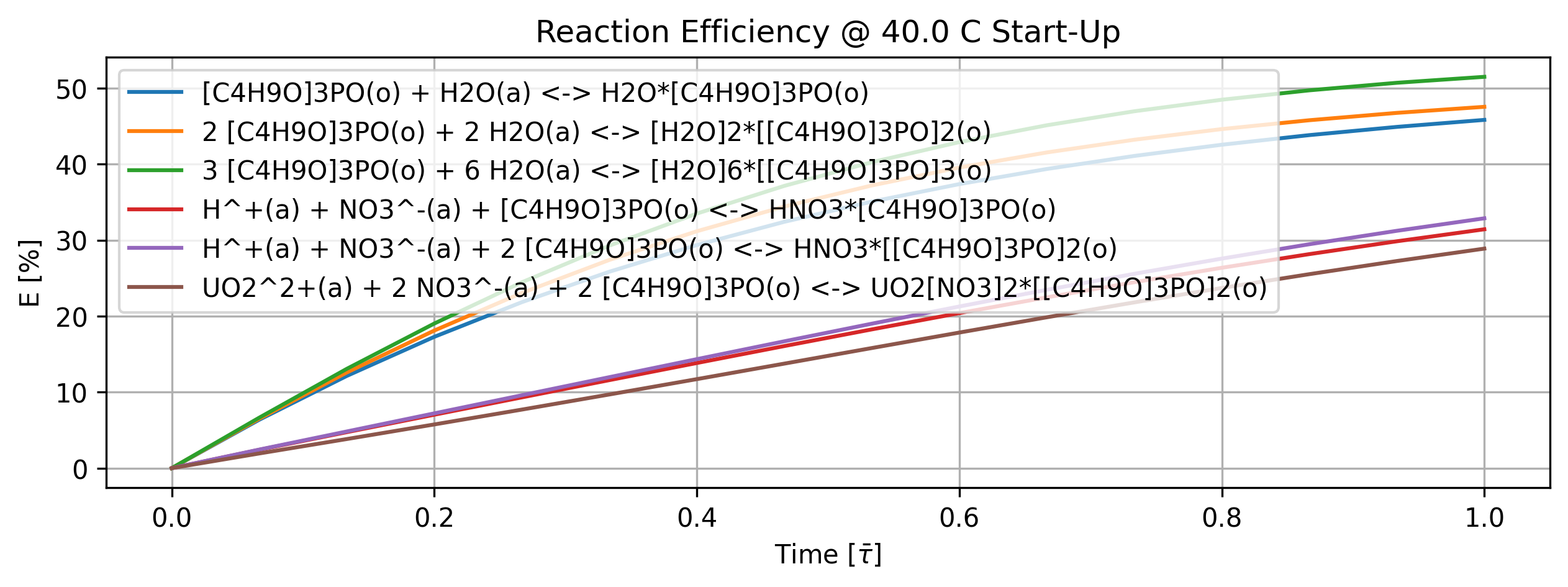
../../_images/b129280a6777c7446d133bc3b07d1c268d413a9648922a01d72164dd98a7308d.png

Figure 6: Reaction efficiency history at start-up.

'''Individual reaction efficiency'''

quant = stg.efficiency_history()

tbl_count += 1
print(f'Table {tbl_count}: Reaction efficiency history at start-up.')
print('Time [min]    Rxn Eff. [%]')

col_names = [f'r{i}' for i in range(len(stg.rxn_mech.reactions))]
time_name = ''
df = (quant.value.apply(pd.Series).mul(1)
       .rename(index=lambda i: round(i/unit.min,2))
       .set_axis(col_names, axis=1).rename_axis(time_name)
       .round(3))
print(df.to_string(max_rows=20, min_rows=20))

Table 4: Reaction efficiency history at start-up.
Time [min]    Rxn Eff. [%]
          r0      r1      r2      r3      r4      r5
                                                    
00   0.000   0.000   0.000   0.000   0.000   0.000
06   6.372   6.507   6.645   2.418   2.445   1.934
12  12.135  12.589  13.066   4.736   4.827   3.830
18  17.277  18.105  19.026   7.031   7.209   5.751
24  21.835  23.048  24.451   9.311   9.590   7.704
30  25.843  27.393  29.272  11.579  11.969   9.692
36  29.350  31.169  33.491  13.833  14.340  11.711
42  32.408  34.418  37.137  16.062  16.691  13.752
48  35.066  37.193  40.254  18.256  19.007  15.801
55  37.369  39.548  42.895  20.397  21.271  17.840
61  39.360  41.537  45.112  22.472  23.464  19.849
67  41.076  43.209  46.955  24.464  25.568  21.810
73  42.551  44.609  48.473  26.363  27.571  23.705
79  43.816  45.774  49.708  28.160  29.459  25.522
85  44.898  46.741  50.700  29.848  31.227  27.250
91  45.819  47.540  51.486  31.426  32.871  28.882

if cortix_ai:
    issues = '+ Title your reponse as: Overview of Individual Reaction Efficiency at Start-Up.'
    cortix_ai.explain(quant=quant, issues=issues, markdown_header_level='<h4>', markdown_display=markdown_display, save_supporting_info=db_save, print_prompt=False)

Cortix AI assistant: working on explanation...

Overview of Individual Reaction Efficiency at Start-Up

Data summary

The table records reaction efficiencies (percent) for six ordered reactions sampled at eight times from 0 s to 50.9091 s (steps ≈ 7.2727 s).
All six reaction columns start at 0% (t = 0) and rise monotonically through the recorded start‑up interval.

Mapping of columns to reactions

Column 0: [C₄H₉O]₃PO(o) + H₂O(a) <=> H₂O·[C₄H₉O]₃PO(o)
Column 1: 2 [C₄H₉O]₃PO(o) + 2 H₂O(a) <=> [H₂O]₂·[[C₄H₉O]₃PO]₂(o)
Column 2: 3 [C₄H₉O]₃PO(o) + 6 H₂O(a) <=> [H₂O]₆·[[C₄H₉O]₃PO]₃(o)
Column 3: H⁺(a) + NO₃⁻(a) + [C₄H₉O]₃PO(o) <=> HNO₃·[C₄H₉O]₃PO(o)
Column 4: H⁺(a) + NO₃⁻(a) + 2 [C₄H₉O]₃PO(o) <=> HNO₃·[[C₄H₉O]₃PO]₂(o)
Column 5: UO₂²⁺(a) + 2 NO₃⁻(a) + 2 [C₄H₉O]₃PO(o) <=> UO₂[NO₃]₂·[[C₄H₉O]₃PO]₂(o)

Per-reaction numerical trends (start -> final at 50.9091 s)

Reaction (col 0): 0% -> 44.8975%; mean growth ≈ 0.882 %/s; strictly increasing at each sample.
Reaction (col 1): 0% -> 46.7415%; mean growth ≈ 0.918 %/s; strictly increasing.
Reaction (col 2): 0% -> 50.7004%; mean growth ≈ 0.996 %/s; strictly increasing and the largest absolute efficiency.
Reaction (col 3): 0% -> 29.8483%; mean growth ≈ 0.586 %/s; strictly increasing.
Reaction (col 4): 0% -> 31.2270%; mean growth ≈ 0.614 %/s; strictly increasing.
Reaction (col 5): 0% -> 27.2498%; mean growth ≈ 0.535 %/s; strictly increasing.

Comparative observations

The three water‑adduct formation reactions (columns 0–2) exhibit the highest efficiencies and fastest average growth rates, with the 3:6 water adduct (col 2) the largest by the end of the window.
The acid/nitrate and uranyl complexation reactions (columns 3–5) rise more slowly and reach substantially lower efficiencies in the same period.
Among the latter, the single‑ligand HNO₃ adduct (col 3) and the double‑ligand HNO₃ adduct (col 4) are slightly higher than the UO₂ complex (col 5) at final time.

Conclusions

During start‑up the system shows monotonic, roughly linear increases in reaction efficiency on this time scale; water complexation dominates early efficiency gains (col 2 highest).
Sampling is uniform (~7.27 s intervals) and suffices to resolve the steady, monotonic build in each reaction over the first ~51 s.

AI Parameters:
+ LLM model (OpenAI) = gpt-5-mini
+ LLM cleverness     = 1.0
+ Total # of tokens  = 6553

1.5.4. Reaction Rate Density#

This quantity only makes sense per volume of the mixture.

'''Reaction rate density'''
import matplotlib.pyplot as plt

quant = stg.r_vec_history() # mole/m^3-s

quant.plot(title='Reaction Rate Density @ %2.1f C Start-Up'%unit.convert_temperature(stg_temperature,
           'K','C'), x_scaling=1/stg.flow_residence_time_avg, x_label=r'Time [$\bar{\tau}$]', y_label=quant.latex_name+
           ' ['+quant.unit+']', legend=stg.rxn_mech.reactions, show=True, figsize=[10,3], error_data=False)

fig_count += 1
print(f'Figure {fig_count}: Reaction rate density history at start-up.')

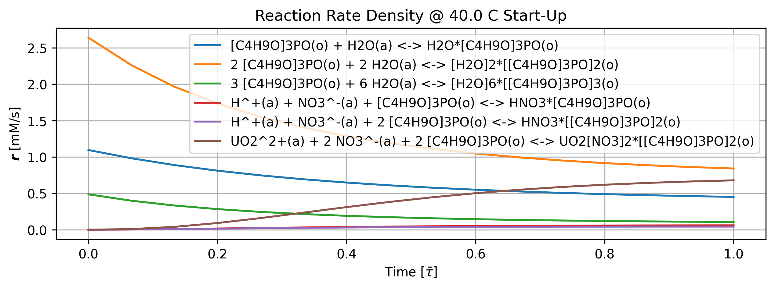
../../_images/98f114cfb90df237a5bda4751505d716b0706111cf319dfa298bf0c5a9dfc5be.png

Figure 7: Reaction rate density history at start-up.

tbl_count += 1
print(f'Table {tbl_count}: Reaction rate density history at start-up.')
print('Time [min]      r [mM/s]')
import pandas as pd
col_names = [f'r{i}' for i in range(len(stg.rxn_mech.reactions))]
time_name = 't [min]'
df = (quant.value.apply(pd.Series).mul(1)
       .rename(index=lambda i: round(i/unit.min,2))
       .set_axis(col_names, axis=1).rename_axis(time_name)
       .round(4))
print(df.to_string(max_rows=20, min_rows=20))

Table 5: Reaction rate density history at start-up.
Time [min]      r [mM/s]
             r0      r1      r2      r3      r4      r5
t [min]                                                
00     1.0955  2.6403  0.4865  0.0000  0.0000  0.0000
06     0.9819  2.2624  0.3985  0.0029  0.0028  0.0082
12     0.8885  1.9663  0.3326  0.0088  0.0080  0.0392
18     0.8115  1.7363  0.2831  0.0160  0.0141  0.0919
24     0.7473  1.5521  0.2446  0.0235  0.0200  0.1595
30     0.6935  1.4047  0.2146  0.0306  0.0255  0.2346
36     0.6482  1.2861  0.1909  0.0369  0.0301  0.3103
42     0.6099  1.1900  0.1720  0.0424  0.0338  0.3818
48     0.5775  1.1118  0.1568  0.0469  0.0367  0.4461
55     0.5498  1.0478  0.1445  0.0505  0.0389  0.5018
61     0.5262  0.9952  0.1344  0.0534  0.0404  0.5486
67     0.5061  0.9518  0.1263  0.0555  0.0414  0.5871
73     0.4889  0.9160  0.1196  0.0572  0.0421  0.6184
79     0.4742  0.8863  0.1141  0.0584  0.0424  0.6434
85     0.4616  0.8617  0.1096  0.0592  0.0425  0.6632
91     0.4508  0.8412  0.1059  0.0598  0.0425  0.6789

if cortix_ai:
    issues = '+ Title your reponse as: Overview of Reaction Rates Density at Start-Up.'
    cortix_ai.explain(quant=quant, issues=issues, markdown_header_level='<h4>', markdown_display=markdown_display, save_supporting_info=db_save, print_prompt=False)

Cortix AI assistant: working on explanation...

Overview of Reaction Rates Density at Start-Up.

Data and context

Time history from 0 to 50.9091 s sampled every 7.2727 s. Dependent quantity: reaction rates density in mM/s for six ordered reactions (columns 0..5 correspond to the reactions listed below, in the same order).

Reaction mapping (converted to chemical-format rules):
- [C₄H₉O]₃PO(o) + H₂O(a) <=> H₂O·[C₄H₉O]₃PO(o)
- 2 [C₄H₉O]₃PO(o) + 2 H₂O(a) <=> [H₂O]₂·[[C₄H₉O]₃PO]₂(o)
- 3 [C₄H₉O]₃PO(o) + 6 H₂O(a) <=> [H₂O]₆·[[C₄H₉O]₃PO]₃(o)
- H⁺(a) + NO₃⁻(a) + [C₄H₉O]₃PO(o) <=> HNO₃·[C₄H₉O]₃PO(o)
- H⁺(a) + NO₃⁻(a) + 2 [C₄H₉O]₃PO(o) <=> HNO₃·[[C₄H₉O]₃PO]₂(o)
- UO₂²⁺(a) + 2 NO₃⁻(a) + 2 [C₄H₉O]₃PO(o) <=> UO₂[NO₃]₂·[[C₄H₉O]₃PO]₂(o)

Overall summary

Early times (t = 0): columns 1, 0, and 2 are the dominant rate contributions (2.64031, 1.09551, 0.486462 mM/s respectively); columns 3–5 are effectively zero (10⁻⁶ mM/s).
Over the 0–50.9 s window columns 0–2 monotonically decrease; columns 3–5 monotonically increase.
Largest relative growth: column 5 (reaction 6) increases by ≈6.0×10⁵-fold (from 1.11×10⁻⁶ to 0.663201 mM/s). Columns 3 and 4 grow ≈1.10×10⁴-fold and ≈8.04×10³-fold respectively.
Largest absolute decreases: column 1 falls from 2.64031 to 0.861679 mM/s (≈67% decrease). Column 0 and 2 fall by ≈58% and ≈77%, respectively.
At final time (50.9091 s) column 1 remains the single largest rate (0.861679 mM/s), followed by column 5 (0.663201 mM/s) and column 0 (0.461584 mM/s).

Column-by-column analysis

Column 0 — [C₄H₉O]₃PO + H₂O -> solvated complex (first solvation step)
- t=0: 1.09551 mM/s; t=50.91 s: 0.461584 mM/s.
- Behavior: monotonic decrease (≈0.42× initial, −57.9%).
- Interpretation (data-only): initially important, decreasing significance over the time window.
Column 1 — 2 [C₄H₉O]₃PO + 2 H₂O -> larger solvated dimer
- t=0: 2.64031 mM/s; t=50.91 s: 0.861679 mM/s.
- Behavior: monotonic decrease (≈0.33× initial, −67.4%).
- Interpretation (data-only): remains the largest single-rate process throughout the sampled period.
Column 2 — 3 [C₄H₉O]₃PO + 6 H₂O -> trimer solvate
- t=0: 0.486462 mM/s; t=50.91 s: 0.109569 mM/s.
- Behavior: monotonic decrease (≈0.23× initial, −77.5%).
- Interpretation (data-only): contribution becomes small by the end of the window.
Column 3 — protonated nitrate complexation to form HNO₃·[C₄H₉O]₃PO
- t=0: 5.38343×10⁻⁶ mM/s; t=50.91 s: 0.0592107 mM/s.
- Behavior: monotonic increase (≈1.10×10⁴-fold).
- Interpretation (data-only): negligible at start, becomes a measurable contributor by ~50 s.
Column 4 — protonated nitrate with dimer: HNO₃·[[C₄H₉O]₃PO]₂
- t=0: 5.28724×10⁻⁶ mM/s; t=50.91 s: 0.0425051 mM/s.
- Behavior: monotonic increase (≈8.04×10³-fold) with growth slowing toward the end (rates begin to level off after ~36–51 s).
Column 5 — UO₂ complex formation UO₂[NO₃]₂·[[C₄H₉O]₃PO]₂
- t=0: 1.10587×10⁻⁶ mM/s; t=50.91 s: 0.663201 mM/s.
- Behavior: monotonic, very large relative increase (≈6.0×10⁵-fold).
- Interpretation (data-only): fastest relative activation; by the end it is a major rate term (second-largest absolute rate).

Concluding remarks

The dataset shows a clear shift in dominant contributions: initial dominance by columns 1–0–2 (solvation steps) and progressive activation of columns 5–4–3 (complexation/ion-pair formation), with column 1 remaining the largest absolute rate across the sampled period.
Time sampling is uniform at ≈7.2727 s intervals; trends are monotonic for each column within the sampled window.

AI Parameters:
+ LLM model (OpenAI) = gpt-5-mini
+ LLM cleverness     = 1.0
+ Total # of tokens  = 7127

1.5.5. Species Generation Rate Density#

This quantity is on the basis of mixing volume so all species generation values can be compared.

'''Species generation rate density'''
import matplotlib.pyplot as plt

quant = stg.g_vec_history() # mole/m^3-s

quant.plot(title='Species Generation Rate Density @ %2.1f C Start-Up'%unit.convert_temperature(stg_temperature,
           'K','C'), x_scaling=1/stg.flow_residence_time_avg, x_label=r'Time [$\bar{\tau}$]', y_label=quant.latex_name+
           ' ['+quant.unit+']', legend=stg.rxn_mech.species_names, show=True, figsize=[10,3], error_data=False)

fig_count += 1
print(f'Figure {fig_count}: Species generation rate density history at start-up.')

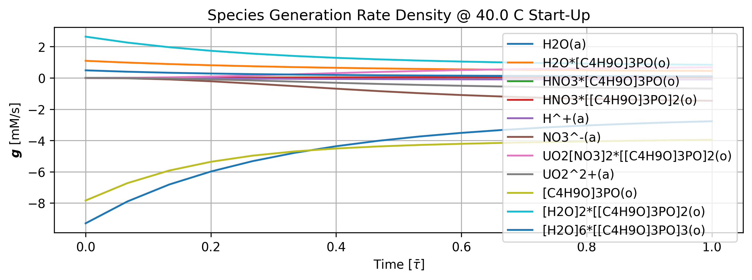
../../_images/a31d3c521da9ebfad32e15416684cc46e3a939ef5cc6f4e04469342003f7720a.png

Figure 8: Species generation rate density history at start-up.

tbl_count += 1
print(f'Table {tbl_count}: Species generation rate density history at start-up.')
print('Time [min]        g [mM/s]')
import pandas as pd
col_names = [f'a{i}' for i in range(len(stg.rxn_mech.species_names))]
time_name = 't [min]'
df = (quant.value.apply(pd.Series).mul(1)
       .rename(index=lambda i: round(i/unit.min,2))
       .set_axis(col_names, axis=1).rename_axis(time_name)
       .round(4))
print(df.to_string(max_rows=20, min_rows=20))

Table 6: Species generation rate density history at start-up.
Time [min]        g [mM/s]
             a0      a1      a2      a3      a4      a5      a6      a7      a8      a9     a10
t [min]                                                                                        
00    -9.2949  1.0955  0.0000  0.0000 -0.0000 -0.0000  0.0000 -0.0000 -7.8355  2.6403  0.4865
06    -7.8975  0.9819  0.0029  0.0028 -0.0057 -0.0220  0.0082 -0.0082 -6.7269  2.2624  0.3985
12    -6.8163  0.8885  0.0088  0.0080 -0.0169 -0.0953  0.0392 -0.0392 -5.9219  1.9663  0.3326
18    -5.9825  0.8115  0.0160  0.0141 -0.0301 -0.2138  0.0919 -0.0919 -5.3612  1.7363  0.2831
24    -5.3192  0.7473  0.0235  0.0200 -0.0435 -0.3626  0.1595 -0.1595 -4.9679  1.5521  0.2446
30    -4.7907  0.6935  0.0306  0.0255 -0.0560 -0.5252  0.2346 -0.2346 -4.6974  1.4047  0.2146
36    -4.3659  0.6482  0.0369  0.0301 -0.0670 -0.6876  0.3103 -0.3103 -4.5109  1.2861  0.1909
42    -4.0220  0.6099  0.0424  0.0338 -0.0762 -0.8398  0.3818 -0.3818 -4.3797  1.1900  0.1720
48    -3.7417  0.5775  0.0469  0.0367 -0.0836 -0.9758  0.4461 -0.4461 -4.2840  1.1118  0.1568
55    -3.5121  0.5498  0.0505  0.0389 -0.0894 -1.0929  0.5018 -0.5018 -4.2106  1.0478  0.1445
61    -3.3232  0.5262  0.0534  0.0404 -0.0938 -1.1910  0.5486 -0.5486 -4.1513  0.9952  0.1344
67    -3.1672  0.5061  0.0555  0.0414 -0.0970 -1.2713  0.5871 -0.5871 -4.1012  0.9518  0.1263
73    -3.0382  0.4889  0.0572  0.0421 -0.0992 -1.3360  0.6184 -0.6184 -4.0575  0.9160  0.1196
79    -2.9312  0.4742  0.0584  0.0424 -0.1007 -1.3875  0.6434 -0.6434 -4.0188  0.8863  0.1141
85    -2.8424  0.4616  0.0592  0.0425 -0.1017 -1.4281  0.6632 -0.6632 -3.9843  0.8617  0.1096
91    -2.7686  0.4508  0.0598  0.0425 -0.1023 -1.4600  0.6789 -0.6789 -3.9534  0.8412  0.1059

'''Produced species generation rate density'''
import matplotlib.pyplot as plt

ids, quant_produced = stg.g_vec_history(produced=True) # mole/m^3-s

quant_produced.plot(title='Produced Species Generation Rate Density @ %2.1f C Start-Up'%unit.convert_temperature(stg_temperature,
           'K','C'), x_scaling=1/stg.flow_residence_time_avg, x_label=r'Time [$\bar{\tau}$]', y_label=quant.latex_name+
           ' ['+quant_produced.unit+']', legend=list(np.array(stg.rxn_mech.species_names)[ids]), show=True, figsize=[10,3], error_data=False)

fig_count += 1
print(f'Figure {fig_count}: Produced species generation rate density history at start-up.')

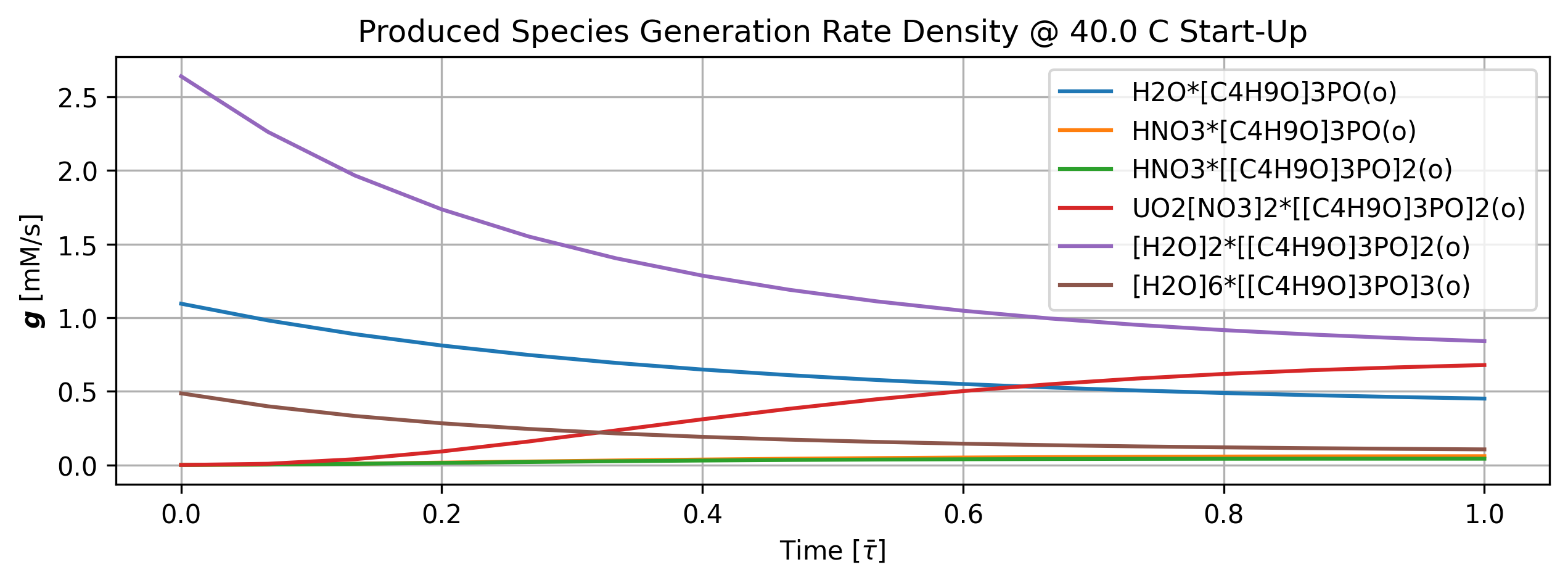
../../_images/6684fc77270d222854fe7e7576185622ef262c62169fa539d0fb34ef930f4b58.png

Figure 9: Produced species generation rate density history at start-up.

if cortix_ai:
    issues = '+ Title your reponse as: Overview of Species Generation Rates Density at Start-Up.'
    cortix_ai.explain(quant=quant, issues=issues, markdown_header_level='<h4>', markdown_display=markdown_display, save_supporting_info=db_save, print_prompt=False)

Cortix AI assistant: working on explanation...

Overview of Species Generation Rates Density at Start-Up

Dataset: generation-rate density time history (dependent unit: mM/s) for 11 ordered species; times (s): 0, 7.27273, 14.5455, 21.8182, 29.0909, 36.3636, 43.6364, 50.9091. Values shown are per-row species rates at those times.

H₂O(a): initial −9.2949 mM/s (0 s) -> −2.84236 mM/s (50.9091 s); negative throughout and increases monotonically toward zero (consumption magnitude decreases).
H₂O·[C₄H₉O]₃PO(o): initial 1.09551 mM/s -> 0.461584 mM/s; positive throughout and decreases monotonically (production decreases).
HNO₃·[C₄H₉O]₃PO(o): initial 5.38343e‑06 mM/s -> 0.0592107 mM/s; starts near zero and increases monotonically to modest positive production.
HNO₃·[[C₄H₉O]₃PO]₂(o): initial 5.28724e‑06 mM/s -> 0.0425051 mM/s; similar behavior to the previous HNO₃ adduct—near zero then monotonic rise in production.
H⁺(a): initial −1.06707e‑05 mM/s -> −0.101716 mM/s; negative throughout and becomes more negative monotonically (increasing net consumption).
NO₃⁻(a): initial −1.28824e‑05 mM/s -> −1.42812 mM/s; negative throughout and magnitude grows monotonically (increasing consumption).
UO₂[NO₃]₂·[[C₄H₉O]₃PO]₂(o): initial 1.10587e‑06 mM/s -> 0.663201 mM/s; positive and increases monotonically (growing production in organic complex).
UO₂²⁺(a): initial −1.10587e‑06 mM/s -> −0.663201 mM/s; negative and decreases monotonically (growing aqueous depletion). Values of this aqueous UO₂²⁺ are equal in magnitude and opposite in sign to the previous organic complex at every time step (direct transfer/stoichiometric pairing).
[C₄H₉O]₃PO(o): initial −7.83553 mM/s -> −3.98427 mM/s; negative throughout and increases monotonically toward zero (consumption magnitude decreases).
[H₂O]₂·[[C₄H₉O]₃PO]₂(o): initial 2.64031 mM/s -> 0.861679 mM/s; positive and decreases monotonically (production declines).
[H₂O]₆·[[C₄H₉O]₃PO]₃(o): initial 0.486462 mM/s -> 0.109569 mM/s; positive and decreases monotonically.

Summary observations: all species show monotonic trends across the sampled start-up window. Several pairs reveal stoichiometric/opposite behavior (notably UO₂ complex in organic phase vs UO₂²⁺ in aqueous phase with exact opposite signs), indicating phase transfer/complexation dynamics. Major magnitudes are seen for H₂O(a) and [C₄H₉O]₃PO(o) (strong net consumption) and for NO₃⁻(a) (growing consumption), while many organic-bound water and adduct species exhibit decreasing production as the system approaches the later times.

AI Parameters:
+ LLM model (OpenAI) = gpt-5-mini
+ LLM cleverness     = 1.0
+ Total # of tokens  = 6264

1.5.6. Mass Balance Residual#

This is actually the total mass generation rate density (mixing volume) residual; a small number in view of total mass conservation.

'''Mass balance residuals'''
import matplotlib.pyplot as plt

quant = stg.mass_balance_residual_history()

quant.plot(title='Total Mass Generation Rate Density @ %2.1f C Start-Up'%unit.convert_temperature(stg_temperature,
           'K','C'), x_scaling=1/stg.flow_residence_time_avg, x_label=r'Time [$\bar{\tau}$]', y_label=quant.latex_name+
           ' ['+quant.unit+']', markers_only=True, legend=['Residual'], show=True, figsize=[10,3])

fig_count += 1
print(f'Figure {fig_count}: Total mass generation rate density residual history at start-up.')

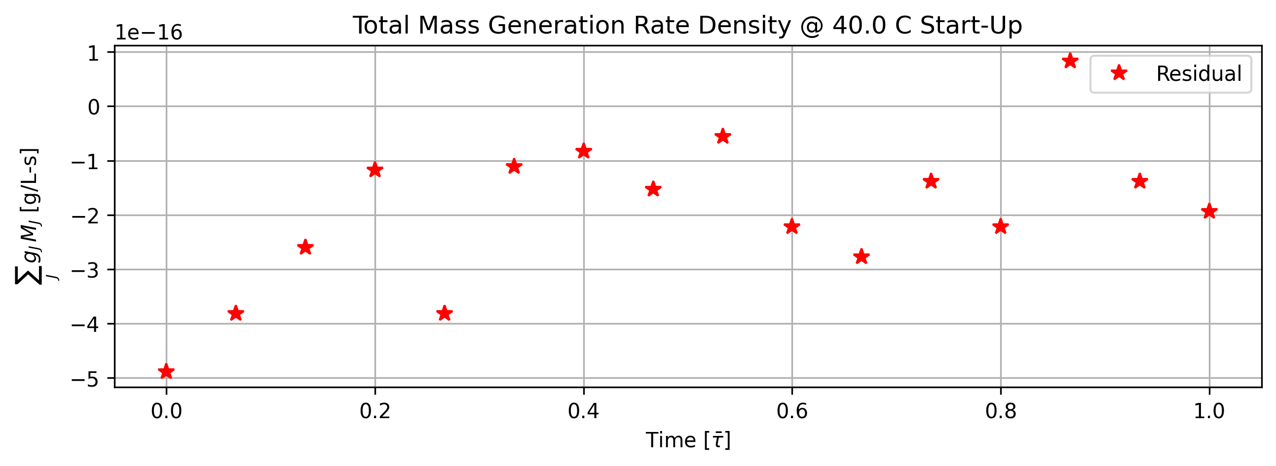
../../_images/922dde669dd832df3b3c4c2968fd085c8e955b3bed745157f132bbdaadb034bc.png

Figure 10: Total mass generation rate density residual history at start-up.

if cortix_ai:
    issues = '+ Title your reponse as: Total Mass Generation Rate Density Residual at Start-Up.'
    cortix_ai.explain(quant=quant, issues=issues, markdown_header_level='<h4>', markdown_display=markdown_display, save_supporting_info=db_save, print_prompt=False)

Cortix AI assistant: working on explanation...

Total Mass Generation Rate Density Residual at Start-Up.

Summary

The table reports the total mass generation rate density (mass balance residual) in the mixing volume at eight times during start-up. The residuals are consistently negative and of order 10⁻¹⁶ g·L⁻¹·s⁻¹, i.e., at or below typical double‑precision round‑off.

Sample count: 8 time samples.
Time range: 0 s to 50.9091 s (uniform spacing ≈ 7.27273 s).
Residual range: minimum = -4.88649·10⁻¹⁶ g·L⁻¹·s⁻¹, maximum = -5.55112·10⁻¹⁷ g·L⁻¹·s⁻¹.
Mean residual: -2.228 × 10⁻¹⁶ g·L⁻¹·s⁻¹.
Root-mean-square (RMS): 2.734 × 10⁻¹⁶ g·L⁻¹·s⁻¹.
Population standard deviation: 1.584 × 10⁻¹⁶ g·L⁻¹·s⁻¹.
Maximum absolute residual (magnitude): 4.88649 × 10⁻¹⁶ g·L⁻¹·s⁻¹.

Data columns analyzed

time [s]: timestamps at which the residual was evaluated; values are 0, 7.27273, 14.5455, 21.8182, 29.0909, 36.3636, 43.6364, 50.9091 s.
Total Mass Generation Rate Density [g/L-s]: instantaneous mass balance residuals (negative values shown), given in g·L⁻¹·s⁻¹.

Interpretation

All residual values are essentially zero within numerical precision (10⁻¹⁶ g·L⁻¹·s⁻¹). The mean and RMS quantify small systematic bias (mean ≈ -2.2·10⁻¹⁶) and typical fluctuation scale (RMS ≈ 2.7·10⁻¹⁶).
The sign (negative) indicates a tiny net sink in the computed mixing-volume balance at these times, but the magnitude is negligible relative to physically meaningful mass fluxes and consistent with round‑off/error levels for double‑precision arithmetic.

AI Parameters:
+ LLM model (OpenAI) = gpt-5-mini
+ LLM cleverness     = 1.0
+ Total # of tokens  = 4615

1.6. Steady-State Simulation#

Pick up from where it left from the past run() and continue to a longer time. This demonstrates how to continue a simulation from where it was interrupted. Note that the state of the system is automatically used as the initial condition for the next run().

end_time += 5 * stg.flow_residence_time_avg
time_step = 5 * stg.flow_residence_time_avg / 15
show_time = (True, 10*time_step)

stg.time_step = time_step
stg.initial_time = stg.end_time
stg.end_time = end_time
stg.show_time = show_time

'''Run system in parallel'''
stg.monitor_mass_flowrates = False
stg.monitor_mass_conservation_residual = False
system.run()
system.close() # Shutdown Cortix

[26493] 2025-12-02 15:23:41,069 - cortix - INFO - Launching Module <solvex.stage.Stage object at 0x7fcf21d59590>
[28594] 2025-12-02 15:23:42,214 - cortix - INFO - Stg-1::run():time[m]=0.9
[28594] 2025-12-02 15:23:42,409 - cortix - INFO - Stg-1::run():time[m]=3.9
Total mass rate density (mixture volume) residual [g/L-s]= -2.77556e-16
total mass inflow rate [g/min]   = 7.418e+02
total mass outflow rate [g/min]  =  7.416e+02
	 net total mass flow rate [g/min] = -1.590e-01
[28594] 2025-12-02 15:23:42,489 - cortix - INFO - Stg-1::run():time[m]=5.5 (et[s]=0.3)
[26493] 2025-12-02 15:23:42,667 - cortix - INFO - run()::Elapsed wall clock time [s]: 714.7
[26493] 2025-12-02 15:23:42,668 - cortix - INFO - Closed Cortix object.
_____________________________________________________________________________
                           T E R M I N A T I N G                             
_____________________________________________________________________________
      ...                                        s       .     (TAAG Fraktur)
   xH88"`~ .x8X                                 :8      @88>
 :8888   .f"8888Hf        u.      .u    .      .88      %8P      uL   ..
:8888>  X8L  ^""`   ...ue888b   .d88B :@8c    :888ooo    .     .@88b  @88R
X8888  X888h        888R Y888r ="8888f8888r -*8888888  .@88u  ""Y888k/"*P
88888  !88888.      888R I888>   4888>"88"    8888    888E`    Y888L
88888   %88888      888R I888>   4888> "      8888      888E      8888
88888 `> `8888>     888R I888>   4888>        8888      888E      `888N
`8888L %  ?888   ! u8888cJ888   .d888L .+    .8888Lu=   888E   .u./"888&
 `8888  `-*""   /   "*888*P"    ^"8888*"     ^%888*     888&  d888" Y888*"
   "888.      :"      "Y"          "Y"         "Y"      R888" ` "Y   Y"
     `""***~"`                                           ""
                             https://cortix.org                              
_____________________________________________________________________________
[26493] 2025-12-02 15:23:42,669 - cortix - INFO - close()::Elapsed wall clock time [s]: 714.7

'''Recover stage'''
stg = system_net.modules[0]

1.6.1. Organic Phase Results#

'''Plot organic phase'''
# TODO: time axis normalized by phase flow residence time.
stg.organic_phase.plot(title='Organic Phase Steady-State', legend='Organic Phase', nrows=2,ncols=3, show=True, figsize=[12,6])

fig_count += 1
print(f'Figure {fig_count}: Organic phase species history dashboard at steady-state.')

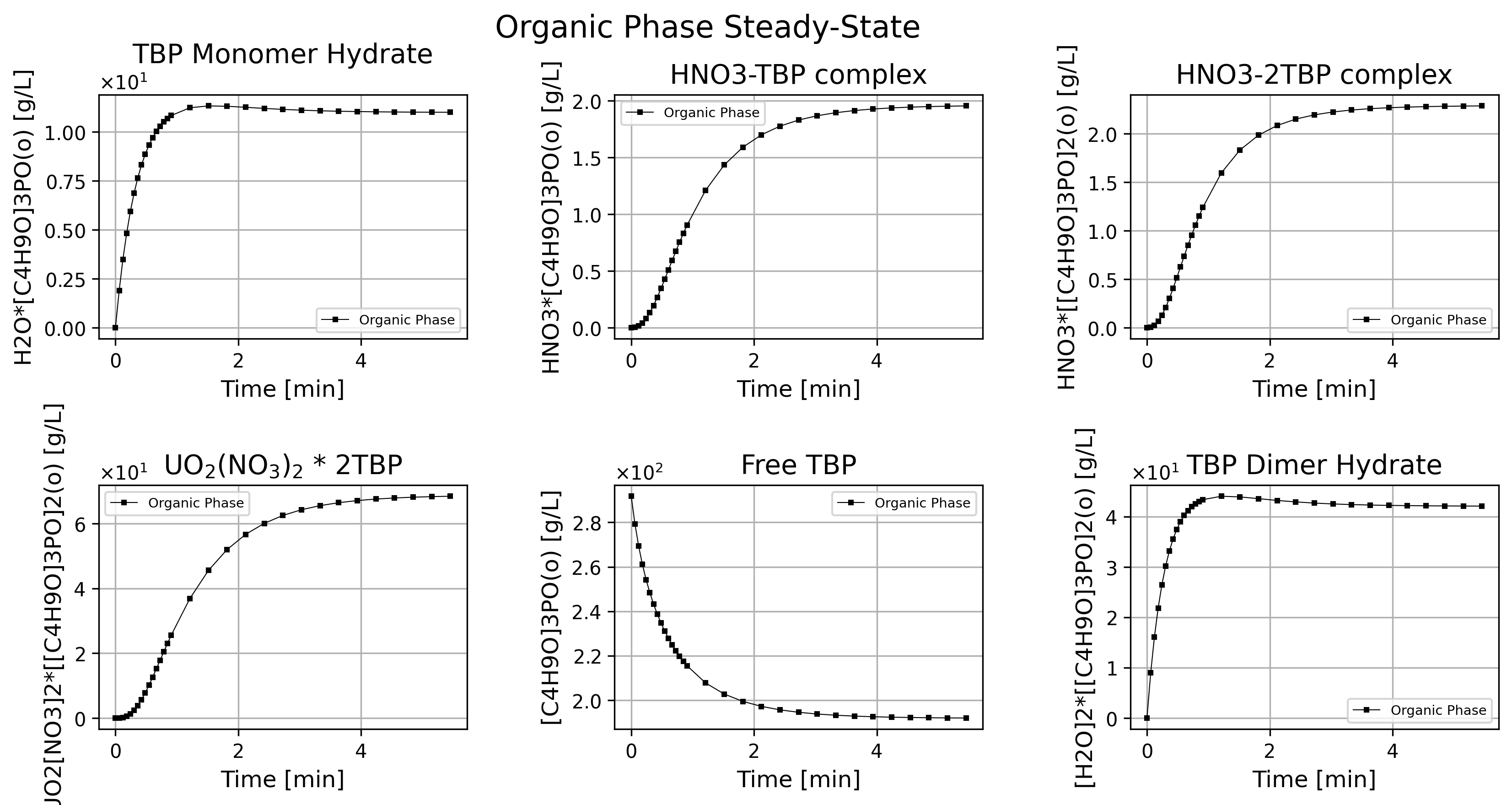
../../_images/b288b0a1a5ade5a6f1eda6fe89a86dd11b0820eb4c930fd8a1a566d7f8619603.png

../../_images/493fc38b17f6ca7e6b5e9e556bc6c31837f8b033e0f12f85575e869799b9b6cd.png

Figure 11: Organic phase species history dashboard at steady-state.

if cortix_ai:
    issues = ('+ Title your reponse as: Overview of the Organic Phase Data at Steady-State.\n'
              '+ Do not explain the start-up process; cover the steady-state only.'
    )
    cortix_ai.explain(phase=stg.organic_phase, markdown_header_level='<h4>', markdown_display=markdown_display, save_supporting_info=db_save)

Cortix AI assistant: working on explanation...

Summary

The dataset records concentrations (g/L) vs time (s) for one free organic, [C₄H₉O]₃PO(o), and several organo-associated species formed by association with H₂O, HNO₃, UO₂[NO₃]₂ and additional water-ligand aggregates.
Over 0 → 327.273 s the free [C₄H₉O]₃PO(o) falls substantially while all listed complexes form and either reach a plateau or slow their growth.

Time-series highlights (per column)

time (s)
- Measurements span 0 to 327.273 s with non-uniform sampling, denser early (< 60 s) and sparser later.
H₂O·[C₄H₉O]₃PO(o)
- 0 → 11.0056 g/L (final). Rapid initial rise in the first ~40 s (≈10 g/L) then approaches ~11.0 g/L (small further increase to ≈11.33 at 90.9 s then slight decline to 11.0056).
HNO₃·[C₄H₉O]₃PO(o)
- 0 → 1.95395 g/L (final). Monotonic increase, leveling toward ~1.95–1.95 range after ≈200 s.
HNO₃·[[C₄H₉O]₃PO]₂(o)
- 0 → 2.28548 g/L (final). Grows faster than the single-ligand HNO₃ complex initially, then slows and approaches ≈2.28.
UO₂[NO₃]₂·[[C₄H₉O]₃PO]₂(o)
- 0 → 68.3955 g/L (final). Largest absolute increase; growth is substantial early and continues rising throughout the record, approaching ~68 g/L by 327 s.
[C₄H₉O]₃PO(o) (free organic)
- 291.75 → 191.977 g/L (final). Net decrease ≈99.77 g/L, a ≈34.2% reduction from initial, indicating the free organic is being consumed/partitioned into complexes.
[H₂O]₂·[[C₄H₉O]₃PO]₂(o)
- 0 → 42.0769 g/L (final). Rapid rise to ~44 g/L by ~55 s, then gradual decline to ≈42.08 by 327 s (small net decrease from peak).
[H₂O]₆·[[C₄H₉O]₃PO]₃(o)
- 0 → 8.14239 g/L (final). Peaks near ~10.22 g/L around 50–55 s then decreases to ~8.14 g/L by 327 s.

Comparative behavior and relative magnitudes

Largest absolute sink: UO₂[NO₃]₂·[[C₄H₉O]₃PO]₂(o) reaches ≈68.4 g/L, the single-largest complex concentration at final time.
The free organic ([C₄H₉O]₃PO(o)) remains the largest single-species pool throughout but declines by ~34%, consistent with substantial transfer into complexes.
Water-containing aggregates:
- [H₂O]₂·[[C₄H₉O]₃PO]₂(o) attains the next-largest concentrations (~42 g/L final) and shows a peak then mild decrease.
- [H₂O]₆·[[C₄H₉O]₃PO]₃(o) is smaller (final ≈8.14 g/L) and shows a clear early peak then decay.
Acid-associated species:
- HNO₃·[[C₄H₉O]₃PO]₂(o) (≈2.29 g/L) and HNO₃·[C₄H₉O]₃PO(o) (≈1.95 g/L) remain minor in mass compared with the uranium and water complexes but show clear formation and leveling.

Kinetics / qualitative rates (early vs long-term)

Early-phase (0–40 s): rapid formation of H₂O·[C₄H₉O]₃PO(o) (~10 g/L in 40 s), UO₂-complex (~15 g/L in 40 s) and [H₂O]₂·[[C₄H₉O]₃PO]₂(o) (~41 g/L by 54.5 s). This indicates fast initial complexation/partitioning.
Later-phase (>100 s): most species’ growth slows and approaches quasi-steady values (plateaus or slow continued rise), e.g., H₂O·[C₄H₉O]₃PO(o) ≈11.0, HNO₃ complexes ≈1.9–2.3, UO₂-complex ≈68–68.4 (still slowly rising).
Some complexes exhibit a peak then slight decline (notably [H₂O]₆·[[C₄H₉O]₃PO]₃(o) and [H₂O]₂·[[C₄H₉O]₃PO]₂(o) around 50–75 s), suggesting redistribution among species or transient maxima.

Notable quantitative points

Free [C₄H₉O]₃PO(o): initial 291.75 g/L → final 191.977 g/L (Δ = −99.773 g/L, −34.2%).
UO₂[NO₃]₂·[[C₄H₉O]₃PO]₂(o): final ≈68.3955 g/L, largest formed complex mass.
H₂O·[C₄H₉O]₃PO(o): rises quickly to ≈11 g/L and then stabilizes (peak ≈11.33 g/L).
HNO₃-associated species remain small (<2.3 g/L each) relative to water and UO₂ complexes.

Concise interpretation

The table shows conversion of free [C₄H₉O]₃PO(o) into multiple associated species on the timescale 0–327 s. The dominant sink by mass is formation of the UO₂-containing complex and water-associated aggregates, while nitrate–acid complexes form in much smaller amounts and level off earlier. Overall dynamics are fast initially and approach steady-state-like values by a few hundred seconds.

AI Parameters:
+ LLM model (OpenAI) = gpt-5-mini
+ LLM cleverness     = 1.0
+ Total # of tokens  = 6814

'''Organic phase mass density'''
import matplotlib.pyplot as plt

quant = stg.mass_density_history('organic')

quant.plot(title='Organic Phase Mass Density @ %2.1f C Steady-State'%unit.convert_temperature(stg_temperature,
           'K','C'), x_scaling=1/stg.flow_residence_time_avg, x_label=r'Time [$\bar{\tau}$]', y_label=quant.latex_name+r'$-\rho_\text{diluent}$'+
           ' ['+quant.unit+']', show=True, figsize=[10,3], error_data=False)

fig_count += 1
print(f'Figure {fig_count}: Organic phase mass density history at steady-state.')

../../_images/c3f1f0667bc9db0ac0ef1d9e6292a84d2bf13d46a539f1d6ceb9aeb8423ab11f.png

Figure 12: Organic phase mass density history at steady-state.

tbl_count += 1
print(f'Table {tbl_count}: Organic phase mass density history at steady-state.')
print('Time [s]  Organic Phase Mass Density [g/L]')
print(quant.value[::5].apply(lambda x: round(x,2)))

Table 7: Organic phase mass density history at steady-state.
Time [s]  Organic Phase Mass Density [g/L]
000000      291.75
181818     296.10
363636     301.65
545455     307.60
454545    322.35
363636    325.28
272727    325.84
Name: Organic Phase Mass Density [g/L]; Time History in [s], dtype: float64

1.6.2. Aqueous Phase Results#

'''Plot aqueous phase'''
# TODO: time axis normalized by phase flow residence time.
stg.aqueous_phase.plot(title='Aqueous Phase Steady-State', legend='Aqueous Phase', nrows=2,ncols=3, show=True, figsize=[12,6])

fig_count += 1
print(f'Figure {fig_count}: Aqueous phase species history dashboard at steady-state.')

../../_images/2b6d0ac089238be17290d165536f12743abe10857668d315abd96cb02a18a9fd.png

Figure 13: Aqueous phase species history dashboard at steady-state.

if cortix_ai:
    issues = ('+ Title your reponse as: Overview of the Aqueous Phase Data at Steady-State.\n'
              '+ Do not explain the start-up process; cover the steady-state only.'
    )
    cortix_ai.explain(phase=stg.aqueous_phase, markdown_header_level='<h4>', markdown_display=markdown_display, save_supporting_info=db_save, print_prompt=False)

Cortix AI assistant: working on explanation...

Summary

The table shows time-series aqueous concentrations (g/L) for H₂O(a), H⁺(a), NO₃⁻(a) and UO₂²⁺(a) from t = 0 to t = 327.273 s. H⁺, NO₃⁻ and UO₂²⁺ rise monotonically (large relative increases); H₂O falls slightly early and then levels off near a new, lower value.

Key numbers
H₂O(a): 992.000 -> 986.800 g/L (Δ = −5.200 g/L)
H⁺(a): 0.001007 -> 0.490639 g/L (Δ = +0.489632 g/L)
NO₃⁻(a): 0.062006 -> 19.2306 g/L (Δ = +19.1686 g/L)
UO₂²⁺(a): 0.000000 -> 85.7313 g/L (Δ = +85.7313 g/L)

Trends and monotonicity

Overall behavior
H⁺(a), NO₃⁻(a), UO₂²⁺(a) increase monotonically across the entire time span.
H₂O(a) decreases strongly at first (until ~70 s) then shows a slight recovery/stabilization; the net change is a modest decrease (~0.5% of initial).

Rates (approximate)

Average rate over 0 -> 327.273 s
H₂O(a): −5.200 / 327.273 ≈ −0.0159 g·L⁻¹·s⁻¹
H⁺(a): +0.489632 / 327.273 ≈ +0.00150 g·L⁻¹·s⁻¹
NO₃⁻(a): +19.1686 / 327.273 ≈ +0.0586 g·L⁻¹·s⁻¹
UO₂²⁺(a): +85.7313 / 327.273 ≈ +0.2621 g·L⁻¹·s⁻¹
Early (0 -> 3.63636 s) instantaneous rates (first interval)
H₂O(a): −1.193 / 3.63636 ≈ −0.328 g·L⁻¹·s⁻¹
H⁺(a): +0.032403 / 3.63636 ≈ +0.00891 g·L⁻¹·s⁻¹
NO₃⁻(a): +1.99200 / 3.63636 ≈ +0.548 g·L⁻¹·s⁻¹
UO₂²⁺(a): +7.08898 / 3.63636 ≈ +1.949 g·L⁻¹·s⁻¹
Comment on rates
Rates are much higher at the beginning and then decline, indicating a fast initial input/formation followed by slowing approach toward a plateau for each solute.

Correlations, ratios and mass change

Pairwise behavior
NO₃⁻(a) and UO₂²⁺(a) rise together throughout the record (strong positive co‑variation).
H⁺(a) also increases in parallel but at much smaller absolute concentration.
H₂O(a) decreases as the solutes accumulate (net dilution/consumption effect on water concentration).
Representative ratios (final values)
UO₂²⁺(a) / NO₃⁻(a) ≈ 85.7313 / 19.2306 ≈ 4.46 (final mass-concentration ratio)
Total aqueous concentration (sum of columns) increases by ≈ +100.19 g/L from start to finish (initial ≈ 992.063 g/L, final ≈ 1092.253 g/L), i.e., an added total aqueous mass concentration of ≈ 100.19 g/L.

Approach to steady state and notable points

The increase in NO₃⁻ and UO₂²⁺ slows substantially after ~200 s; by 200–327 s the concentrations change only marginally (evidence of approach toward a new steady/regime).
H₂O(a) reaches a shallow minimum (~986.388 g/L at ~72.7 s) and then drifts up slightly to 986.800 g/L by 327.3 s.
All solute profiles are smooth and monotonic (no oscillations or reversals), consistent with a controlled addition/formation process followed by equilibration.

Concise takeaway

The dataset documents rapid early introduction/formation of NO₃⁻ and UO₂²⁺ with concomitant proton increase and a small net loss of H₂O concentration; after an early transient the system slows and approaches a near steady state by ~200–327 s.

AI Parameters:
+ LLM model (OpenAI) = gpt-5-mini
+ LLM cleverness     = 1.0
+ Total # of tokens  = 7218

'''Aqueous phase mass density'''
import matplotlib.pyplot as plt

quant = stg.mass_density_history('aqueous')

quant.plot(title='Aqueous Phase Mass Density @ %2.1f C Steady-State'%unit.convert_temperature(stg_temperature,
           'K','C'), x_scaling=1/stg.flow_residence_time_avg, x_label=r'Time [$\bar{\tau}$]', y_label=quant.latex_name+
           ' ['+quant.unit+']', show=True, figsize=[10,3], error_data=False)

fig_count += 1
print(f'Figure {fig_count}: Aqueous phase mass density history at Steady-State.')

../../_images/a0b30d9eccf587e0e7e302c71ae1ba6c3a6c96c468e44ddfbaca1833e9f3612f.png

Figure 14: Aqueous phase mass density history at Steady-State.

tbl_count += 1
print(f'Table {tbl_count}: Aqueous phase mass density history at steady-state.')
print('Time [s]  Aqueous Phase Mass Density [g/L]')
print(quant.value[::5].apply(lambda x: round(x,2)))

Table 8: Aqueous phase mass density history at steady-state.
Time [s]  Aqueous Phase Mass Density [g/L]
000000       992.06
181818     1026.94
363636     1049.00
545455     1062.45
454545    1086.96
363636    1091.41
272727    1092.25
Name: Aqueous Phase Mass Density [g/L]; Time History in [s], dtype: float64

1.6.3. Overall Stage Efficiency#

'''Stage overall efficiency'''

quant = stg.efficiency_history(mean=True)
quant.plot(title='Stage Efficiency @ %2.1f C Steady-State'%unit.convert_temperature(stg_temperature,
           'K','C'), x_scaling=1/stg.flow_residence_time_avg, x_label=r'Time [$\bar{\tau}$]', y_label=quant.latex_name+
           ' ['+quant.unit+']', show=True, figsize=[10,3], error_data=True)

fig_count += 1
print(f'Figure {fig_count}: Stage efficiency history steady-state.')

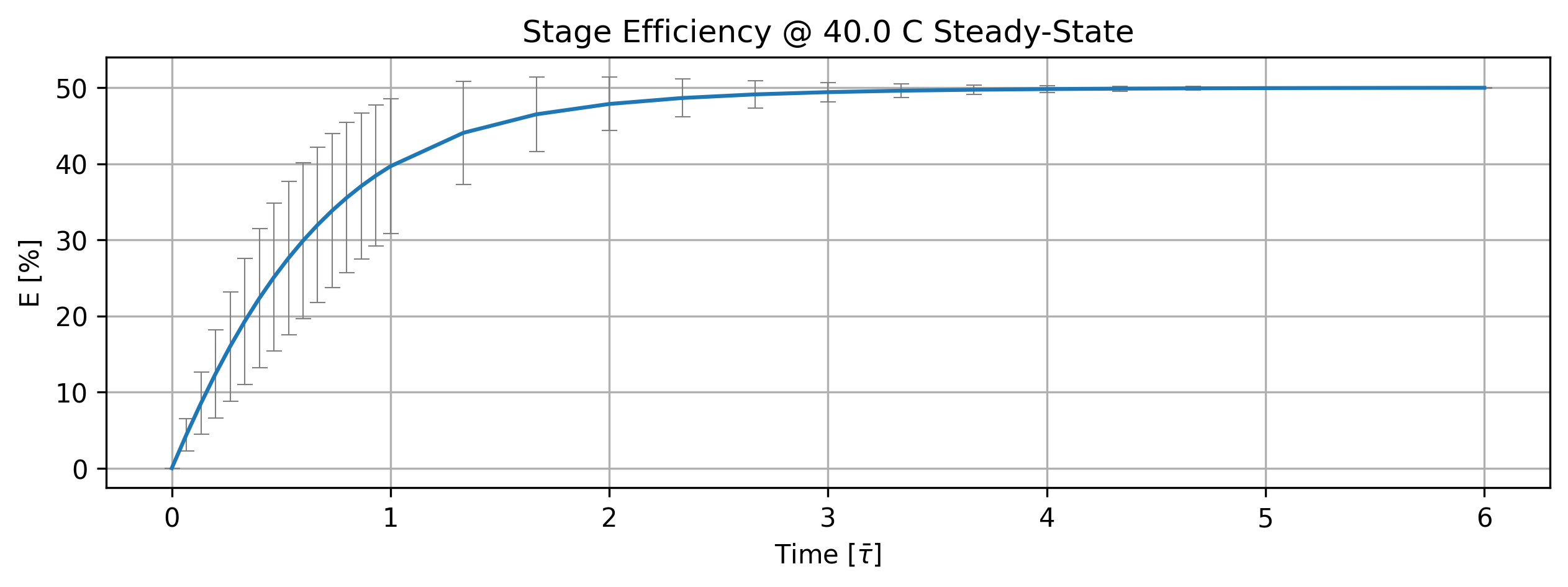
../../_images/3dc55c36a2374dbfa75c99f40d04162318541ef8611d802272f69ddcf65fad1c.png

Figure 15: Stage efficiency history steady-state.

tbl_count += 1
print(f'Table {tbl_count}: Stage efficiency history at steady-state.')
print('Time [s]  (Stage. Eff., +-std) [%]')
time_name = ''
import pandas as pd
df = (quant.value.apply(pd.Series).mul(1)
       .rename(index=lambda i: round(i/unit.min,2))
       .set_axis(['',''], axis=1).rename_axis(time_name)
       .round(3))
print(df.to_string(max_rows=20, min_rows=20))

Table 9: Stage efficiency history at steady-state.
Time [s]  (Stage. Eff., +-std) [%]
                    
                    
00   0.000   0.000
06   4.387   2.129
12   8.530   4.088
18  12.400   5.777
24  15.990   7.185
30  19.291   8.301
36  22.316   9.136
42  25.078   9.715
48  27.596  10.069
55  29.887  10.230
...      ...     ...
73  49.406   1.255
03  49.596   0.891
33  49.722   0.634
64  49.807   0.451
94  49.864   0.322
24  49.904   0.230
55  49.932   0.164
85  49.952   0.117
15  49.966   0.084
45  49.976   0.060

if cortix_ai:
    issues = ('+ Title your reponse as: Overview of the Stage Efficiency Data at Steady-State.\n'
              '+ Do not explain the start-up process; cover the steady-state only.'
    )
    cortix_ai.explain(quant=quant, issues=issues, markdown_header_level='<h4>', markdown_display=markdown_display, save_supporting_info=db_save)

Cortix AI assistant: working on explanation...

Overview of the Stage Efficiency Data at Steady-State.

Steady-state region considered: rows 6–10 (time ≥ 109.091 s). Analysis below covers the time [s], mean efficiency [%] (column “0”), and reported standard deviation [%] (column “1”) for those rows only.

Key steady-state observations

Mean efficiency values settle in the narrow range 47.8515% to 49.9756% (rows 6–10).
Reported standard deviation falls monotonically from 3.51989% at 109.091 s to 0.060092% at 327.273 s, indicating rapidly diminishing variability.
Time sampling in the steady window is regular: 109.091, 163.636, 218.182, 272.727, 327.273 s (interval ≈ 54.545 s).
Final recorded state at 327.273 s: mean = 49.9756%, std = 0.060092%.

Quantitative summary

Mean of the steady-state means (rows 6–10): 49.3944% (arithmetic average of 47.8515, 49.4061, 49.8065, 49.9323, 49.9756).
Sample standard deviation across those five mean values: ≈ 0.80 percentage points.
Reduction in reported pointwise variability from first to last steady sample: factor ≈ 58.6 (3.51989 / 0.060092), corresponding to a ≈ 98.3% decrease in reported std.
Steady-state window duration: 327.273 s − 109.091 s = 218.182 s; five measurement instants evenly spaced within that window.

Summary statement

Over the steady-state window (≥ 109.091 s) the stage efficiency stabilizes near 49.4% on average, with per-sample variability collapsing to near-zero by the last measurement (49.9756% ± 0.0601%).

AI Parameters:
+ LLM model (OpenAI) = gpt-5-mini
+ LLM cleverness     = 1.0
+ Total # of tokens  = 4939

'''Individual reaction efficiency'''

quant = stg.efficiency_history()
quant.plot(title='Reaction Efficiency @ %2.1f C Steady-State'%unit.convert_temperature(stg_temperature,
           'K','C'), x_scaling=1/stg.flow_residence_time_avg, x_label=r'Time [$\bar{\tau}$]', y_label=quant.latex_name+
           ' ['+quant.unit+']', legend=stg.rxn_mech.reactions, show=True, figsize=[10,3])

fig_count += 1
print(f'Figure {fig_count}: Reaction efficiency history at steady-state.')

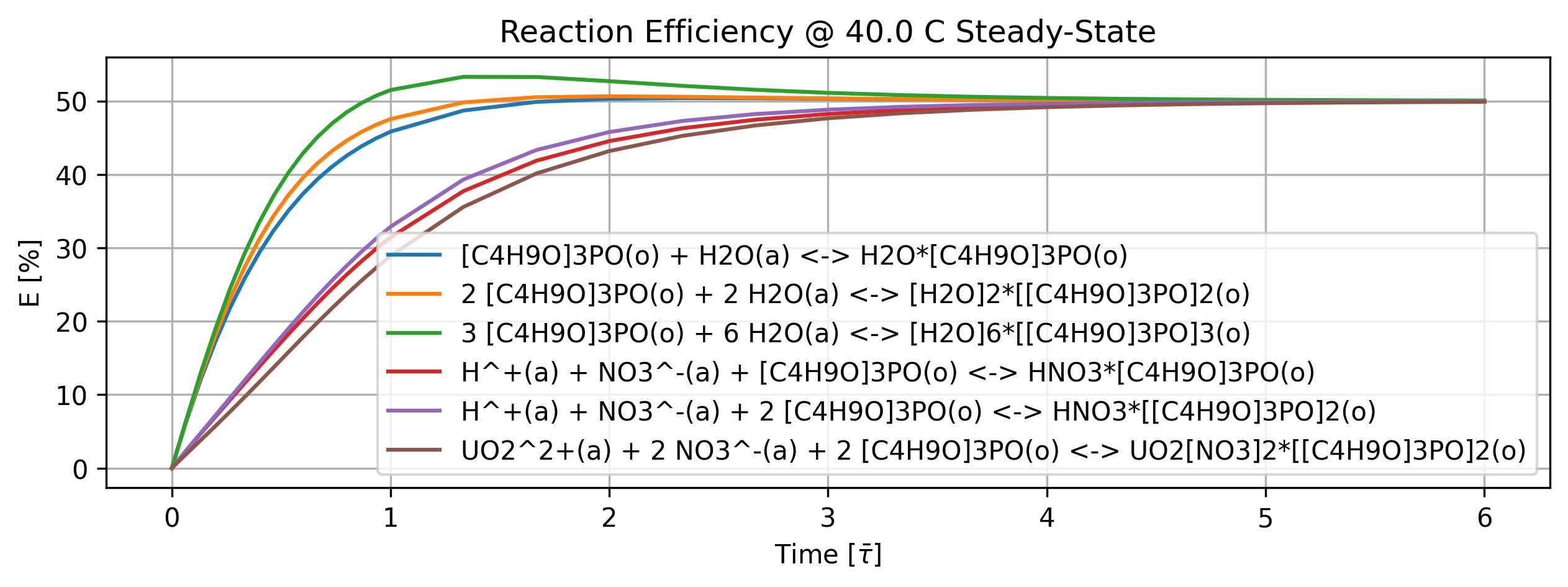
../../_images/897f3af2374144b50bf82fc7deb76e296cf30967ee0947e2b89e596f1dbdbc1e.png

Figure 16: Reaction efficiency history at steady-state.

'''Individual reaction efficiency'''
quant = stg.efficiency_history()
tbl_count += 1
print(f'Table {tbl_count}: Reaction efficiency history at steady-state.')
print('Time [min]    Rxn Eff. [%]')

col_names = [f'r{i}' for i in range(len(stg.rxn_mech.reactions))]
time_name = ''
df = (quant.value.apply(pd.Series).mul(1)
       .rename(index=lambda i: round(i/unit.min,2))
       .set_axis(col_names, axis=1).rename_axis(time_name)
       .round(3))
print(df.to_string(max_rows=20, min_rows=20))

Table 10: Reaction efficiency history at steady-state.
Time [min]    Rxn Eff. [%]
          r0      r1      r2      r3      r4      r5
                                                    
00   0.000   0.000   0.000   0.000   0.000   0.000
06   6.372   6.507   6.645   2.418   2.445   1.934
12  12.135  12.589  13.066   4.736   4.827   3.830
18  17.277  18.105  19.026   7.031   7.209   5.751
24  21.835  23.048  24.451   9.311   9.590   7.704
30  25.843  27.393  29.272  11.579  11.969   9.692
36  29.350  31.169  33.491  13.833  14.340  11.711
42  32.408  34.418  37.137  16.062  16.691  13.752
48  35.066  37.193  40.254  18.256  19.007  15.801
55  37.369  39.548  42.895  20.397  21.271  17.840
...      ...     ...     ...     ...     ...     ...
73  50.305  50.351  51.105  48.227  48.810  47.639
03  50.239  50.261  50.795  48.760  49.197  48.326
33  50.181  50.192  50.570  49.128  49.451  48.809
64  50.135  50.140  50.408  49.384  49.621  49.151
94  50.099  50.101  50.292  49.564  49.737  49.394
24  50.072  50.073  50.208  49.690  49.816  49.567
55  50.052  50.053  50.149  49.779  49.870  49.690
85  50.038  50.038  50.107  49.842  49.908  49.778
15  50.027  50.027  50.076  49.887  49.935  49.841
45  50.020  50.020  50.055  49.920  49.954  49.886

if cortix_ai:
    issues = ('+ Title your reponse as: Overview of Individual Reaction Efficiency at Steady-State'
             '+ Do not explain the start-up process; cover the steady-state only.'
    )
    cortix_ai.explain(quant=quant, issues=issues, markdown_header_level='<h4>', markdown_display=markdown_display, save_supporting_info=db_save)

Cortix AI assistant: working on explanation...

Overview of Individual Reaction Efficiency at Steady-State+ Do not explain the start-up process; cover the steady-state only.

Steady-state window

Steady-state is taken as the final five time points (time [s] = 109.091, 163.636, 218.182, 272.727, 327.273). Reported quantity: reaction efficiency [%]. The table columns 0–5 map to the six ordered reactions supplied.

Per-reaction steady-state summary

Reaction 0 — [C4H9O]3PO(o) + H2O(a) <-> H2O*[C4H9O]3PO(o): mean = 50.161% (min 50.0195, max 50.305), final (327.273 s) = 50.0195%; absolute range = 0.286% (≈0.57% of mean). Stable about 50.16%.
Reaction 1 — 2 [C4H9O]3PO(o) + 2 H2O(a) <-> [H2O]2*[[C4H9O]3PO]2(o): mean = 50.241% (min 50.0196, max 50.6408), final = 50.0196%; range = 0.621% (≈1.24% of mean). Small variability; converged near 50%.
Reaction 2 — 3 [C4H9O]3PO(o) + 6 H2O(a) <-> [H2O]6*[[C4H9O]3PO]3(o): mean = 50.882% (min 50.0546, max 52.6925), final = 50.0546%; range = 2.638% (≈5.18% of mean). Larger settling from a higher interim value; final ≈50.05%.
Reaction 3 — H⁺(a) + NO3⁻(a) + [C4H9O]3PO(o) <-> HNO3*[C4H9O]3PO(o): mean = 48.369% (min 44.5359, max 49.9196), final = 49.9196%; range = 5.384% (≈11.13% of mean). Steady-state close to 49.92% with notable rise across the window.
Reaction 4 — H⁺(a) + NO3⁻(a) + 2 [C4H9O]3PO(o) <-> HNO3*[[C4H9O]3PO]2(o): mean = 48.805% (min 45.7689, max 49.9538), final = 49.9538%; range = 4.185% (≈8.57% of mean). Approaches ~49.95% at final time.
Reaction 5 — UO2²⁺(a) + 2 NO3⁻(a) + 2 [C4H9O]3PO(o) <-> UO2[NO3]2*[[C4H9O]3PO]2(o): mean = 47.909% (min 43.1786, max 49.8864), final = 49.8864%; range = 6.708% (≈14.01% of mean). Largest variability over the steady-state window but final value ≈49.89%.

Aggregate observation

Final snapshot (327.273 s) shows all six reaction efficiencies tightly clustered between 49.886% and 50.055% (spread ≈0.168 percentage points), i.e., effectively ~50% at steady-state.
Early points inside the chosen steady-state window show greater variability for reactions 2–5, but by the final times every reaction converges to approximately 50% efficiency.

AI Parameters:
+ LLM model (OpenAI) = gpt-5-mini
+ LLM cleverness     = 1.0
+ Total # of tokens  = 6607

1.6.4. Reaction Rate Density#

This quantity only makes sense per volume of the mixture.

'''Reaction rate density'''
import matplotlib.pyplot as plt

quant = stg.r_vec_history()# mole/m^3-s

quant.plot(title='Reaction Rate Density @ %2.1f C Steady-State'%unit.convert_temperature(stg_temperature,
           'K','C'), x_scaling=1/stg.flow_residence_time_avg, x_label=r'Time [$\bar{\tau}$]', y_label=quant.latex_name+
           ' ['+quant.unit+']', legend=stg.rxn_mech.reactions, show=True, figsize=[10,3], error_data=False)

fig_count += 1
print(f'Figure {fig_count}: Reaction rate density history at steady-state.')

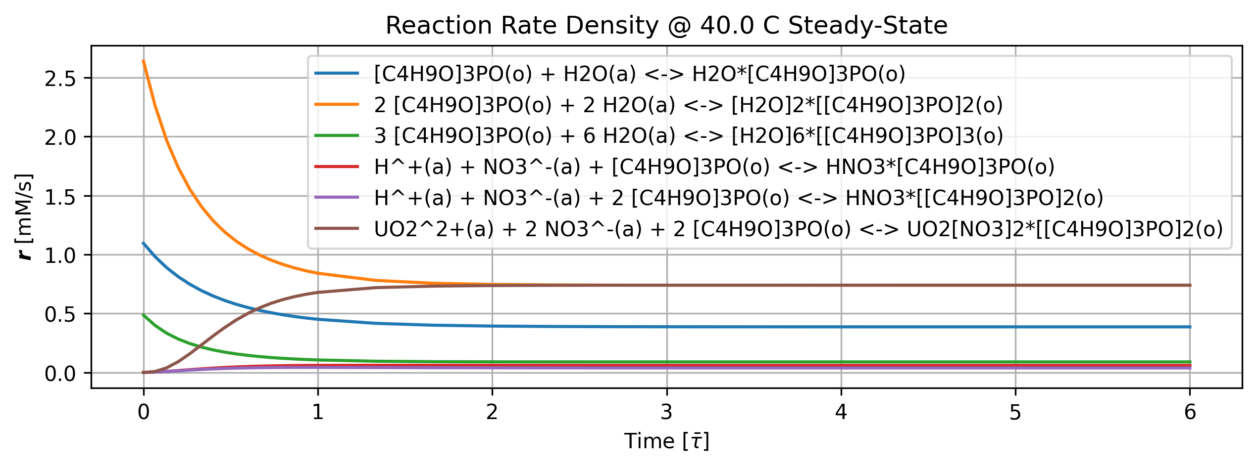
../../_images/4c245aa5f4493269984ccb15043ceee0b713b082e479cb992a6d22a271376cde.png

Figure 17: Reaction rate density history at steady-state.

tbl_count += 1
print(f'Table {tbl_count}: Reaction rate density history at steady-state.')
print('Time [min]      r [mM/s]')
import pandas as pd
col_names = [f'r{i}' for i in range(len(stg.rxn_mech.reactions))]
time_name = 't [min]'
df = (quant.value.apply(pd.Series).mul(1)
       .rename(index=lambda i: round(i/unit.min,2))
       .set_axis(col_names, axis=1).rename_axis(time_name)
       .round(4))
print(df.iloc[n_startup:].to_string(max_rows=20, min_rows=20))

Table 11: Reaction rate density history at steady-state.
Time [min]      r [mM/s]
             r0      r1      r2      r3      r4      r5
t [min]                                                
21     0.4164  0.7805  0.0953  0.0607  0.0414  0.7194
52     0.4006  0.7562  0.0914  0.0605  0.0402  0.7322
82     0.3933  0.7464  0.0901  0.0601  0.0395  0.7369
12     0.3899  0.7424  0.0897  0.0599  0.0390  0.7388
42     0.3883  0.7407  0.0896  0.0597  0.0388  0.7397
73     0.3875  0.7400  0.0895  0.0596  0.0386  0.7401
03     0.3871  0.7397  0.0895  0.0596  0.0385  0.7402
33     0.3869  0.7395  0.0896  0.0596  0.0385  0.7403
64     0.3869  0.7394  0.0896  0.0595  0.0385  0.7404
94     0.3868  0.7394  0.0896  0.0595  0.0385  0.7404
24     0.3868  0.7394  0.0896  0.0595  0.0384  0.7404
55     0.3868  0.7394  0.0896  0.0595  0.0384  0.7404
85     0.3868  0.7394  0.0896  0.0595  0.0384  0.7404
15     0.3868  0.7394  0.0896  0.0595  0.0384  0.7404
45     0.3868  0.7394  0.0896  0.0595  0.0384  0.7404

if cortix_ai:
    issues = ('+ Title your reponse as: Overview of Reaction Rates Density at Steady-State.\n'
              '+ Do not explain the start-up process; cover the steady-state only.'
)
    cortix_ai.explain(quant=quant, issues=issues, markdown_header_level='<h4>', markdown_display=markdown_display, save_supporting_info=db_save, print_prompt=False)

Cortix AI assistant: working on explanation...

Overview of Reaction Rates Density at Steady-State.

Steady-state window

Steady-state is taken from the late-time portion of the table (times 109.091 s through 327.273 s; rows 6–10). All reported Rxn Rates Density values are in mM/s.

Mapping of columns to ordered reactions

Column 0: [C₄H₉O]₃PO(o) + H₂O(a) <=> H₂O*[C₄H₉O]₃PO(o)
Column 1: 2 [C₄H₉O]₃PO(o) + 2 H₂O(a) <=> [H₂O]₂*[[C₄H₉O]₃PO]₂(o)
Column 2: 3 [C₄H₉O]₃PO(o) + 6 H₂O(a) <=> [H₂O]₆*[[C₄H₉O]₃PO]₃(o)
Column 3: H⁺(a) + NO₃⁻(a) + [C₄H₉O]₃PO(o) <=> HNO₃*[C₄H₉O]₃PO(o)
Column 4: H⁺(a) + NO₃⁻(a) + 2 [C₄H₉O]₃PO(o) <=> HNO₃*[[C₄H₉O]₃PO]₂(o)
Column 5: UO₂²⁺(a) + 2 NO₃⁻(a) + 2 [C₄H₉O]₃PO(o) <=> UO₂[NO₃]₂*[[C₄H₉O]₃PO]₂(o)

Per-reaction steady-state statistics (times 109.091–327.273 s)

Column 0 — [C₄H₉O]₃PO + H₂O <=> H₂O*[C₄H₉O]₃PO
- Mean rate ≈ 0.3882 mM/s
- Standard deviation ≈ 0.00258 mM/s (coefficient of variation ≈ 0.66%)
Column 1 — 2 [C₄H₉O]₃PO + 2 H₂O <=> [H₂O]₂*[[C₄H₉O]₃PO]₂
- Mean rate ≈ 0.7409 mM/s
- Standard deviation ≈ 0.00271 mM/s (CV ≈ 0.37%)
Column 2 — 3 [C₄H₉O]₃PO + 6 H₂O <=> [H₂O]₆*[[C₄H₉O]₃PO]₃
- Mean rate ≈ 0.08967 mM/s
- Standard deviation ≈ 0.00022 mM/s (CV ≈ 0.25%)
Column 3 — H⁺ + NO₃⁻ + [C₄H₉O]₃PO <=> HNO₃*[C₄H₉O]₃PO
- Mean rate ≈ 0.05967 mM/s
- Standard deviation ≈ 0.00023 mM/s (CV ≈ 0.38%)
Column 4 — H⁺ + NO₃⁻ + 2 [C₄H₉O]₃PO <=> HNO₃*[[C₄H₉O]₃PO]₂
- Mean rate ≈ 0.03869 mM/s
- Standard deviation ≈ 0.00042 mM/s (CV ≈ 1.09%)
Column 5 — UO₂²⁺ + 2 NO₃⁻ + 2 [C₄H₉O]₃PO <=> UO₂[NO₃]₂*[[C₄H₉O]₃PO]₂
- Mean rate ≈ 0.7396 mM/s
- Standard deviation ≈ 0.00136 mM/s (CV ≈ 0.18%)

Key steady-state observations

The two largest steady-state rates are Columns 1 and 5 (≈0.741 mM/s and ≈0.740 mM/s); they essentially tie and dominate the rate density.
Column 0 is intermediate (~0.388 mM/s). Columns 2, 3 and 4 are markedly smaller (≈0.0897, 0.0597, 0.0387 mM/s respectively).
Variability across the steady-state window is very small for all reactions (CV mostly << 1%), indicating well-established steady values over 109–327 s.

AI Parameters:
+ LLM model (OpenAI) = gpt-5-mini
+ LLM cleverness     = 1.0
+ Total # of tokens  = 7232

1.6.5. Species Generation Rate Density#

This quantity is on the basis of mixing volume so all species generation values can be compared.

'''Species generation rate density'''
import matplotlib.pyplot as plt

quant = stg.g_vec_history() # mole/m^3-s

quant.plot(title='Species Generation Rate Density @ %2.1f C Steady-State'%unit.convert_temperature(stg_temperature,
           'K','C'), x_scaling=1/stg.flow_residence_time_avg, x_label=r'Time [$\bar{\tau}$]', y_label=quant.latex_name+
           ' ['+quant.unit+']', legend=stg.rxn_mech.species_names, show=True, figsize=[10,3], error_data=False)

fig_count += 1
print(f'Figure {fig_count}: Species generation rate density history at steady-state.')

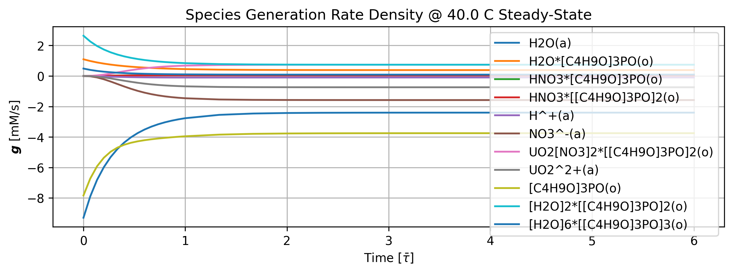
../../_images/70d43cf945641ac9949b05a5d4639fffd86e9da9ccb6f81d2a271fd015aa2b03.png

Figure 18: Species generation rate density history at steady-state.

tbl_count += 1
print(f'Table {tbl_count}: Species generation rate density history at steady-state.')
print('Time [min]        g [mM/s]')
import pandas as pd
col_names = [f'a{i}' for i in range(len(stg.rxn_mech.species_names))]
time_name = 't [min]'
df = (quant.value.apply(pd.Series).mul(1)
       .rename(index=lambda i: round(i/unit.min,2))
       .set_axis(col_names, axis=1).rename_axis(time_name)
       .round(4))
print(df.iloc[n_startup:].to_string(max_rows=20, min_rows=20))

Table 12: Species generation rate density history at steady-state.
Time [min]        g [mM/s]
             a0      a1      a2      a3      a4      a5      a6      a7      a8      a9     a10
t [min]                                                                                        
21    -2.5491  0.4164  0.0607  0.0414 -0.1021 -1.5408  0.7194 -0.7194 -3.8454  0.7805  0.0953
52    -2.4617  0.4006  0.0605  0.0402 -0.1007 -1.5652  0.7322 -0.7322 -3.7928  0.7562  0.0914
82    -2.4268  0.3933  0.0601  0.0395 -0.0996 -1.5734  0.7369 -0.7369 -3.7694  0.7464  0.0901
12    -2.4128  0.3899  0.0599  0.0390 -0.0989 -1.5766  0.7388 -0.7388 -3.7593  0.7424  0.0897
42    -2.4071  0.3883  0.0597  0.0388 -0.0985 -1.5778  0.7397 -0.7397 -3.7550  0.7407  0.0896
73    -2.4047  0.3875  0.0596  0.0386 -0.0983 -1.5784  0.7401 -0.7401 -3.7531  0.7400  0.0895
03    -2.4037  0.3871  0.0596  0.0385 -0.0981 -1.5786  0.7402 -0.7402 -3.7522  0.7397  0.0895
33    -2.4033  0.3869  0.0596  0.0385 -0.0981 -1.5787  0.7403 -0.7403 -3.7518  0.7395  0.0896
64    -2.4031  0.3869  0.0595  0.0385 -0.0980 -1.5788  0.7404 -0.7404 -3.7516  0.7394  0.0896
94    -2.4030  0.3868  0.0595  0.0385 -0.0980 -1.5788  0.7404 -0.7404 -3.7515  0.7394  0.0896
24    -2.4029  0.3868  0.0595  0.0384 -0.0980 -1.5788  0.7404 -0.7404 -3.7515  0.7394  0.0896
55    -2.4029  0.3868  0.0595  0.0384 -0.0980 -1.5788  0.7404 -0.7404 -3.7515  0.7394  0.0896
85    -2.4029  0.3868  0.0595  0.0384 -0.0980 -1.5788  0.7404 -0.7404 -3.7515  0.7394  0.0896
15    -2.4029  0.3868  0.0595  0.0384 -0.0980 -1.5788  0.7404 -0.7404 -3.7515  0.7394  0.0896
45    -2.4029  0.3868  0.0595  0.0384 -0.0980 -1.5788  0.7404 -0.7404 -3.7514  0.7394  0.0896

'''Produced species generation rate density'''
import matplotlib.pyplot as plt

ids, quant_produced = stg.g_vec_history(produced=True) # mole/m^3-s

quant_produced.plot(title='Produced Species Generation Rate Density @ %2.1f C Steady-State'%unit.convert_temperature(stg_temperature,
           'K','C'), x_scaling=1/stg.flow_residence_time_avg, x_label=r'Time [$\bar{\tau}$]', y_label=quant.latex_name+
           ' ['+quant_produced.unit+']', legend=list(np.array(stg.rxn_mech.species_names)[ids]), show=True, figsize=[10,3], error_data=False)

fig_count += 1
print(f'Figure {fig_count}: Produced species generation rate density history at steady-state.')

../../_images/3ab09b8ba9ef6ab45658f10b9740cd363fb2f2b336b6b2772433391f4fa67561.png

Figure 19: Produced species generation rate density history at steady-state.

if cortix_ai:
    issues = ('+ Title your reponse as: Overview of Species Generation Rates Density at Steady-State.\n'
              '+ Do not explain the start-up process; cover the steady-state only.\n'
              '+ Identify the groups of produced species and consumed species.'
)
    cortix_ai.explain(quant=quant, issues=issues, markdown_header_level='<h4>', markdown_display=markdown_display, save_supporting_info=db_save, print_prompt=False)

Cortix AI assistant: working on explanation...

Overview of Species Generation Rates Density at Steady-State.

Steady-state snapshot

At the final time point (steady-state, last row) the per-species generation rates [mM/s] are:

H₂O(a): -2.40292 (consumed)
H₂O·[C₄H₉O]₃PO(o): 0.386769 (produced)
HNO₃·[C₄H₉O]₃PO(o): 0.0595228 (produced)
HNO₃·[[C₄H₉O]₃PO]₂(o): 0.038441 (produced)
H⁺(a): -0.0979638 (consumed)
NO₃⁻(a): -1.57881 (consumed)
UO₂[NO₃]₂·[[C₄H₉O]₃PO]₂(o): 0.740424 (produced)
UO₂²⁺(a): -0.740424 (consumed)
[C₄H₉O]₃PO(o): -3.75145 (consumed)
[H₂O]₂·[[C₄H₉O]₃PO]₂(o): 0.739353 (produced)
[H₂O]₆·[[C₄H₉O]₃PO]₃(o): 0.0895736 (produced)

Produced vs consumed groups (steady-state)

Produced species (positive generation rates):
- H₂O·[C₄H₉O]₃PO(o)
- HNO₃·[C₄H₉O]₃PO(o)
- HNO₃·[[C₄H₉O]₃PO]₂(o)
- UO₂[NO₃]₂·[[C₄H₉O]₃PO]₂(o)
- [H₂O]₂·[[C₄H₉O]₃PO]₂(o)
- [H₂O]₆·[[C₄H₉O]₃PO]₃(o)
Consumed species (negative generation rates):
- H₂O(a)
- H⁺(a)
- NO₃⁻(a)
- UO₂²⁺(a)
- [C₄H₉O]₃PO(o)

Quantitative summary and observations

Total production (sum of positive rates) ≈ 2.05408 mM/s.
- Main contributors: UO₂[NO₃]₂·[[C₄H₉O]₃PO]₂(o) (0.740424, 36.1% of production) and [H₂O]₂·[[C₄H₉O]₃PO]₂(o) (0.739353, 36.0%).
- Secondary contributor: H₂O·[C₄H₉O]₃PO(o) (0.386769, 18.8%).
Total consumption (absolute sum of negative rates) ≈ 8.57157 mM/s.
- Major sinks: [C₄H₉O]₃PO(o) (-3.75145, 43.7% of consumption) and H₂O(a) (-2.40292, 28.0%).
- NO₃⁻(a) is a significant sink (-1.57881, 18.4%).
Net balance at steady-state (production − consumption) ≈ −6.51748 mM/s (net consumption overall).
Notable near-exact internal interconversion: UO₂[NO₃]₂·[[C₄H₉O]₃PO]₂(o) is produced at +0.740424 mM/s while UO₂²⁺(a) is consumed at −0.740424 mM/s, indicating a direct conversion between aqueous UO₂²⁺ and the organophosphate-bound UO₂ complex with essentially no net rate difference at steady-state.

AI Parameters:
+ LLM model (OpenAI) = gpt-5-mini
+ LLM cleverness     = 1.0
+ Total # of tokens  = 6939

1.6.6. Mass Balance Residual#

This is actually the total mass generation rate density (mixing volume) residual; a small number in view of total mass conservation.

'''Mass balance residuals'''
import matplotlib.pyplot as plt

quant = stg.mass_balance_residual_history()

quant.plot(title='Total Mass Generation Rate Density @ %2.1f C Steady-State'%unit.convert_temperature(stg_temperature,
           'K','C'), x_scaling=1/stg.flow_residence_time_avg, x_label=r'Time [$\bar{\tau}$]', y_label=quant.latex_name+
           ' ['+quant.unit+']', markers_only=True, legend=['Residual'], show=True, figsize=[10,3])

fig_count += 1
print(f'Figure {fig_count}: Total mass generation rate density residual history at steady-state.')

../../_images/10bdfd3ce64c055a5627ff2bc3a1b0c85ac7ef93230a0d06c0b4de47a18a636f.png

Figure 20: Total mass generation rate density residual history at steady-state.

if cortix_ai:
    issues = ('+ Title your reponse as: Total Mass Generation Rate Density Residual at Steady-State.\n'
             '+ Do not explain the start-up process; cover the steady-state only.'
    )
    cortix_ai.explain(quant=quant, issues=issues, markdown_header_level='<h4>', markdown_display=markdown_display, save_supporting_info=db_save, print_prompt=False)

Cortix AI assistant: working on explanation...

Total Mass Generation Rate Density Residual at Steady-State.

Overview

Dataset: 11 time samples of “Total Mass Generation Rate Density” with units g/L-s and time in s.
Time column: min = 0 s, max = 327.273 s, number of samples = 11.
Dependent column (steady-state focus): values provided are all negative and have magnitudes on the order of 10⁻¹⁶ g/L-s.

Steady-state subset

Steady-state samples considered: indices 6–10 (times 109.091 s, 163.636 s, 218.182 s, 272.727 s, 327.273 s).
Steady-state values (g/L-s): -2.77556e-17, -5.55112e-17, -1.38778e-16, -2.77556e-17, -2.77556e-16.

Steady-state statistics (numeric)

Mean (steady-state) = -1.05471e-16 g/L-s.
Median = -5.55112e-17 g/L-s.
Minimum = -2.77556e-16 g/L-s (most negative).
Maximum = -2.77556e-17 g/L-s (least negative).
Maximum absolute residual = 2.77556e-16 g/L-s.
Population standard deviation ≈ 3.01e-16 g/L-s.
RMS (steady-state) ≈ 3.01e-16 g/L-s.

Interpretation

All steady-state residuals have magnitudes ≲ 3×10⁻¹⁶ g/L-s, i.e., on the order of 10⁻¹⁶ g/L-s.
These values are consistent with numerical round-off / machine-precision-level residuals for a conserved mass balance evaluated in double precision; they indicate the mass generation rate density is effectively zero at steady-state within numerical noise.

AI Parameters:
+ LLM model (OpenAI) = gpt-5-mini
+ LLM cleverness     = 1.0
+ Total # of tokens  = 5176

1.7. AI Reports#

The Stage AI Report agent builds a Solvex Knowledge Base from the simulation up to this point, and uses it as a retrieval augmented generation (RAG) AI to analyze the results and provide a report.

'''Create and Configure a StageAI Object for a particular stg'''
if stage_ai:
    from stage_ai import StageAI
    stage_ai = StageAI(stg, llm_model='gpt-5-mini', llm_cleverness=0.8)
    stage_ai.n_chunks = 8
    stage_ai.markdown_header_level = '<h4>'

1.7.1. Aqueous Phase#

Request a report from the LLM.

if stage_ai:
    issues = ('+ Title your response as: Aqueous Phase Analysis.\n'
              '+ Discuss in particular, for the aqueous phase, why the simulated steady-state concentration of O2 in the aqueous'
              ' phase is lower than N2 when the solubility of O2 in the aqueous phase is higher than the solubility of N2.\n'
              f'+ Consider stage efficiency only up to {round(stg.initial_time,2)} seconds.'
             )
    stage_ai.report(phase='aqueous', issues=issues, markdown_display=markdown_display, save_supporting_info=db_save, print_prompt=False)

Stage AI assistant: working on report...

Aqueous Phase Analysis

Introduction
This report analyzes the aqueous phase in the provided Stage Knowledge Base (source: stg.aqueous_phase). The system is a two‑liquid (aqueous–organic) extraction/mixing system that tracks aqueous species (water, hydrogen ion, nitrate ion, uranyl ion) and interactions with an organic extractant (tributyl phosphate, TBP). The analysis uses time-series concentration data (units: g/L) and stage information (word “stage” is used where stage data are considered). Stage efficiency is considered only up to 54.55 s as requested.

Data and scope

The Stage Knowledge Base provides: aqueous species properties (molar mass, charge, atom counts), time histories of aqueous species mass concentrations (g/L) at multiple time stamps (s), a reaction mechanism including aqueous–organic complexation reactions, “Stage Efficiency” time history (mean ± std) and stage mass balance residuals (Total Mass Generation Rate Density [g/L-s]) at the same time stamps.

Phases involved: aqueous phase (notation “(a)”) and organic phase (notation “(o)”). Reactions in the mechanism include transfer/complexation between aqueous and organic phases.

Chemical species characteristics
Table 1: Key chemical species in the aqueous phase with phase, charge, molar mass (kg/mol) and atom count.

| Commercial name | Chemical formula (phase) | Charge | Molar mass [kg/mol] | Number of atoms | |—|—:|—:|—:|—:| | Water | H₂O(a) | 0 | 0.018015 | 3 | | Hydrogen ion (proton) | H⁺(a) | +1 | 0.0010074 | 1 | | Nitrate ion | NO₃⁻(a) | −1 | 0.062006 | 4 | | Uranyl ion | UO₂²⁺(a) | +2 | 0.27130 | 3 |

Time‑dependent aqueous concentrations (mass concentration)
Table 2: Time history of aqueous phase species concentrations. Time unit: seconds (s). Concentration unit: grams per liter (g/L).

| Time [s] | Water (H₂O(a)) [g/L] | Hydrogen ion (H⁺(a)) [g/L] | Nitrate ion (NO₃⁻(a)) [g/L] | Uranyl ion (UO₂²⁺(a)) [g/L] | |—:|—:|—:|—:|—:| | 0.0000 | 992.00 | 0.0010074 | 0.062006 | 0.00000 | | 10.910 | 989.11 | 0.091851 | 5.5700 | 19.757 | | 21.820 | 987.65 | 0.16541 | 9.5685 | 34.925 | | 32.730 | 986.92 | 0.22498 | 12.226 | 46.084 | | 43.640 | 986.57 | 0.27341 | 13.970 | 54.319 | | 54.550 | 986.42 | 0.31294 | 15.159 | 60.558 | | 109.09 | 986.53 | 0.42580 | 17.875 | 76.882 | | 163.64 | 986.69 | 0.46750 | 18.755 | 82.602 | | 218.18 | 986.76 | 0.48289 | 19.072 | 84.686 | | 272.73 | 986.79 | 0.48855 | 19.188 | 85.450 | | 327.27 | 986.80 | 0.49064 | 19.231 | 85.731 |

Stage efficiency (considered up to 54.55 s)
Table 3: Stage overall efficiency (mean ± std) expressed in percent. Time unit: seconds (s). Only times ≤ 54.55 s are considered for claims about approach to equilibrium.

| Time [s] | Stage efficiency (mean) [%] | Standard deviation [%] | |—:|—:|—:| | 0.0000 | 0.00000 | 0.00000 | | 10.910 | 12.400 | 5.7800 | | 21.820 | 22.320 | 9.1400 | | 32.730 | 29.890 | 10.230 | | 43.640 | 35.550 | 9.8900 | | 54.550 | 39.670 | 8.8500 |

Interpretation: at 54.55 s the stage efficiency is 39.67% (±8.85%), well below the ~100% that would be required to claim chemical equilibrium on a stage basis. Therefore thermodynamic/chemical equilibrium assumptions are not justified for the time interval considered.

Stage mass balance

The Stage Knowledge Base reports “Total Mass Generation Rate Density [g/L-s]” (mass balance residual) at all time stamps. Values are provided as −0.0 at each timestamp (numerically zero to the reported precision). This indicates that the model’s mass balance for the tracked quantities is effectively conserved within numerical precision for the recorded times. The word “stage” is used explicitly since stage mass and stage efficiency data are reported.

Reaction mechanism involving the aqueous phase
Table 4: Reaction mechanism entries in the Stage Knowledge Base that involve the aqueous phase. Each reaction line below lists the reaction (with phases) and the KB description; an extra explanatory remark follows.

[C₄H₉O]₃PO(o) + H₂O(a) <-> H₂O·[C₄H₉O]₃PO(o)

KB description: complexation of one H2O molecule

Extra information: This reaction is the complexation (solvation) of one aqueous water molecule by one tributyl phosphate (TBP) molecule in the organic phase, forming a TBP–water adduct in the organic phase; it transfers one H₂O from the aqueous phase into a solvated organic adduct (phase involvement: aqueous -> organic).

2 [C₄H₉O]₃PO(o) + 2 H₂O(a) <-> [H₂O]₂·[[C₄H₉O]₃PO]₂(o)

KB description: complexation of two H2O molecules

Extra information: This reaction describes a 2:2 complex where two aqueous water molecules are complexed with two TBP molecules and extracted into the organic phase as a solvated cluster; it is an explicit multi‑molecule solvation/extraction step (aqueous -> organic).

3 [C₄H₉O]₃PO(o) + 6 H₂O(a) <-> [H₂O]₆·[[C₄H₉O]₃PO]₃(o)

KB description: complexation of six H2O molecules

Extra information: Higher order solvation complexation: six water molecules from the aqueous phase coordinate with three TBP molecules in the organic phase forming a larger solvated aggregate; mechanism implies multipoint solvation and larger uptake of water into the organic phase.

H⁺(a) + NO₃⁻(a) + [C₄H₉O]₃PO(o) <-> HNO₃·[C₄H₉O]₃PO(o)

KB description: one TBP complexation of HNO3

Extra information: This reaction is the extraction/complexation of nitric acid (HNO₃ formed from H⁺ + NO₃⁻ in the aqueous phase) by one TBP molecule into the organic phase as a solvated HNO₃·TBP adduct; it is an acid extraction (aqueous acid species -> organic adduct).

H⁺(a) + NO₃⁻(a) + 2 [C₄H₉O]₃PO(o) <-> HNO₃·[[C₄H₉O]₃PO]₂(o)

KB description: two TBP complexation of HNO3

Extra information: Similar to the previous reaction but with two TBP molecules solvating a single HNO₃; this is a stronger/more solvated extraction complex facilitating more efficient acid extraction to the organic phase.

UO₂²⁺(a) + 2 NO₃⁻(a) + 2 [C₄H₉O]₃PO(o) <-> UO₂[NO₃]₂·[[C₄H₉O]₃PO]₂(o)

KB description: uranyl nitrate complexation with 2TBP

Extra information: This reaction is the extraction of aqueous uranyl ion (UO₂²⁺) as the neutral uranyl nitrate complex UO₂(NO₃)₂ which is solvated by two TBP molecules and transferred to the organic phase as a UO₂[NO₃]₂·[[C₄H₉O]₃PO]₂(o) adduct; mechanism explicitly couples aqueous complexation (UO₂²⁺ + NO₃⁻) and organic solvation by TBP.

Notes on the reaction list and mechanism:

All listed reactions involve species in the aqueous phase (H₂O(a), H⁺(a), NO₃⁻(a), UO₂²⁺(a)) and organic extractant [C₄H₉O]₃PO(o); therefore all are pertinent to the aqueous-phase analysis.

Reactions are written preserving phases: (a) = aqueous phase, (o) = organic phase.

Discussion — O₂ vs N₂ dissolved concentrations in the aqueous phase
Context: The Stage Knowledge Base header indicates the presence of air and multiphase behavior, but explicit O₂ and N₂ species concentrations or solubility constants are not provided in the KB data set. The following are mechanistic explanations consistent with the provided stage/kinetic information and general mass‑transfer/thermodynamic principles.

Non‑equilibrium (stage efficiency) argument:

The reported stage efficiency at 54.55 s is 39.67% (±8.85%), substantially below 100%. Under non‑equilibrium conditions, dissolved concentrations are controlled by kinetic mass transfer rates (gas→liquid transfer coefficients and interfacial area) and by reaction/consumption rates, not only by Henry’s‑law solubility.

If the system has insufficient time or insufficient interfacial transfer to reach Henry’s‑law equilibrium, the species with the larger gas‑phase partial pressure and sufficient transfer driving force can end up at higher dissolved concentrations even if its intrinsic solubility (Henry’s constant) is lower.

Gas‑phase partial pressure / driving force:

Air composition (approximate molar fractions: N₂ ≈ 78%, O₂ ≈ 21%) produces a larger bulk partial pressure for N₂ than for O₂. The dissolved concentration under finite mass transfer is proportional to the product of solubility and gas‑phase partial pressure driving force. A larger partial pressure for N₂ can compensate for a lower Henry’s law solubility, yielding higher dissolved N₂ at steady (simulated) conditions that are not at thermodynamic equilibrium.

Chemical consumption of O₂ in the aqueous phase:

Although the KB reactions do not explicitly list O₂ reactions, O₂ is chemically reactive (oxidant) in many aqueous systems. If any unreported side reactions or model components consume dissolved oxygen (oxidation of organics, reduced metal species, or O₂ uptake by extractant complexes), O₂ steady‑state concentration will be depressed relative to N₂. The provided mechanism shows active extraction of nitrate, protons, water and uranyl complexes; those processes change the chemical environment (e.g., acid, redox potentials) and can indirectly influence O₂ solubility and consumption.

Competitive mass transfer or partitioning to the organic phase:

If dissolved O₂ preferentially partitions into the organic phase, or is consumed in the organic phase, its aqueous steady concentration can be lower. The KB explicitly shows water and nitric acid extraction to the organic phase; while O₂ is not explicitly modeled, partitioning/uptake behavior of trace gases could reduce dissolved O₂.

Summary of reasons (consistent with KB and stage data):

The system is not at chemical equilibrium (stage efficiency << 100% up to 54.55 s), so Henry’s law equilibrium cannot be assumed. Under kinetic control, a larger gas‑phase partial pressure of N₂ (air composition) and/or faster transfer of N₂ can result in higher aqueous N₂ than O₂ despite higher O₂ intrinsic solubility.

Additional plausible contributions (not directly present as reactions in the KB) include aqueous or organic phase consumption of O₂ and preferential partitioning of O₂ into the organic phase; either effect reduces aqueous O₂ concentration relative to N₂.

Conclusions

System type: The mixture is a two‑liquid multiphase (aqueous–organic) extraction system (liquid–liquid extraction) with aqueous phase species H₂O(a), H⁺(a), NO₃⁻(a), UO₂²⁺(a) and an organic extractant [C₄H₉O]₃PO(o) (TBP).

Equilibrium: The reported stage efficiencies up to 54.55 s (maximum 39.67% ± 8.85%) are far below 100%, therefore chemical equilibrium on a stage basis is not achieved in the time window considered; predictions should not assume full thermodynamic equilibrium.

Reaction mechanism: The dominant aqueous‑phase relevant mechanisms in the KB are solvation/complexation and extraction of water and nitric acid and the extraction of uranyl nitrate as UO₂(NO₃)₂·(TBP)₂ species into the organic phase. These reactions explicitly couple aqueous ion chemistry (H⁺, NO₃⁻, UO₂²⁺) with organic‑phase solvating TBP.

O₂ vs N₂ aqueous concentration explanation: Given the non‑equilibrium (sub‑100% stage efficiency) state and the larger gas‑phase partial pressure of N₂ in air, N₂ can reach higher simulated aqueous concentrations than O₂ even though O₂ has higher intrinsic aqueous solubility. Additional depletion of O₂ by chemical consumption or partitioning to the organic phase would further lower aqueous O₂ concentration.

Recommendations (succinct)

If resolving the O₂ vs N₂ discrepancy is critical, add explicit species and reactions for dissolved O₂ and N₂ (including Henry’s constants and any chemical/biological consumption paths) and include gas‑phase partial pressures. This will permit direct mass‑transfer and reaction coupling and enable checking whether mass‑transfer kinetics or chemical consumption control dissolved concentrations.

To approach steady‑state/near‑equilibrium behavior, simulate longer times or increase modeled interfacial transfer rates; monitor stage efficiency trends. For robust equilibrium claims do not rely on stage efficiencies < 95–99%.

Data provenance

The analysis is based exclusively on the provided Stage Knowledge Base entry titled “Stage Knowledge Base (Stg-1): aqueous phase” (source key: stg.aqueous_phase). All numerical values (molar masses, mass concentrations, time stamps, stage efficiency, reaction descriptions and reaction strings) are taken from that KB. All phases used are indicated explicitly as (a) for aqueous and (o) for organic in the KB.

AI Parameters:
+ LLM model (OpenAI) = gpt-5-mini
+ LLM cleverness     = 1.0
+ RAG                = stg.aqueous_phase
+ Total # of tokens  = 16603
Done with report...

1.7.2. Organic Phase#

Request a report from the LLM.

if stage_ai:
    issues = ('+ Title your response as: Organic Phase Analysis.\n'
              f'+ Consider stage efficiency only up to {round(stg.initial_time,2)} seconds.'
             )
    stage_ai.report(phase='organic', issues=issues, markdown_display=markdown_display, save_supporting_info=db_save)

Stage AI assistant: working on report...

Organic Phase Analysis

Overview

This report analyzes the organic-phase species, their time-dependent concentrations, and the reaction mechanism from the provided Stage Knowledge Base (source: stg.organic_phase). The system is an aqueous–organic extraction (aqueous phase (a) / organic phase (o)) in which tributyl phosphate (TBP) in the organic phase complexes water, nitric acid, and uranyl nitrate. Stage information (the word “stage” is used in the Stage Knowledge Base) including stage efficiency and mass balance residuals is available and has been used; stage module data are therefore considered in the analysis.

Species characteristics (commercial name, chemical formula, phase, molar mass, atom count)

Species characteristics table.

Time-dependent species data (time series)

Time-dependent concentrations for organic-phase species. Time unit: seconds (s). Concentration units: not specified in the Stage Knowledge Base (KB does not provide explicit concentration units); values are presented as given in the KB and rounded to five significant digits.

| Time [s] | TBP (free) | TBP monohydrate | TBP dimer dihydrate | TBP trimer hexahydrate | HNO₃·TBP (1:1) | HNO₃·(TBP)₂ (1:2) | UO₂(NO₃)₂·(TBP)₂ | |—:|—:|—:|—:|—:|—:|—:|—:| | 0.0000 | 291.75 | 0.00000 | 0.00000 | 0.00000 | 0.00000 | 0.00000 | 0.00000 | | 10.910 | 261.09 | 4.8193 | 21.828 | 6.0327 | 0.039914 | 0.065060 | 0.52025 | | 21.820 | 243.26 | 7.6569 | 33.119 | 8.7198 | 0.19533 | 0.29990 | 3.8192 | | 32.730 | 231.13 | 9.3273 | 38.980 | 9.8429 | 0.42650 | 0.62588 | 10.110 | | 43.640 | 222.20 | 10.296 | 41.948 | 10.202 | 0.67405 | 0.95367 | 17.829 | | 54.550 | 215.49 | 10.840 | 43.352 | 10.191 | 0.90260 | 1.2387 | 25.583 | | 109.090 | 199.46 | 11.313 | 43.549 | 9.1041 | 1.5900 | 1.9844 | 51.964 | | 163.640 | 194.55 | 11.153 | 42.675 | 8.4882 | 1.8296 | 2.1934 | 62.481 | | 218.180 | 192.83 | 11.059 | 42.284 | 8.2570 | 1.9132 | 2.2570 | 66.409 | | 272.730 | 192.21 | 11.020 | 42.133 | 8.1730 | 1.9431 | 2.2781 | 67.861 | | 327.270 | 191.98 | 11.005 | 42.076 | 8.1424 | 1.9539 | 2.2855 | 68.396 |

Stage efficiency (considered only up to 54.55 s)

Stage Efficiency (mean ± std) — time history (units: percent [%]; time unit: seconds). Only the time window up to 54.55 s is used for any thermodynamic-equilibrium claims per instruction.

| Time [s] | Efficiency mean [%] | Efficiency std [%] | |—:|—:|—:| | 0.0000 | 0.00000 | 0.00000 | | 10.910 | 12.400 | 5.7800 | | 21.820 | 22.320 | 9.1400 | | 32.730 | 29.890 | 10.230 | | 43.640 | 35.550 | 9.8900 | | 54.550 | 39.670 | 8.8500 |

Observations on stage efficiency (0–54.55 s):

The stage efficiency rises from 0% at t = 0 to 39.67% at t = 54.55 s (mean values). The standard deviation is appreciable in the early period (≈5.78–10.23 %) and decreases somewhat later.
Because stage efficiency is well below ~100% in the considered window (0–54.55 s), the system cannot be assumed to have reached chemical (thermodynamic) equilibrium; observed species distributions reflect kinetic progression toward extraction equilibrium, not final thermodynamic equilibrium.

Mass balance residuals (stage)

Total mass generation rate density (units: g·L⁻¹·s⁻¹); time unit: seconds. Values in the KB are effectively zero (displayed as -0.0); here they are presented rounded to five significant digits.

| Time [s] | Mass balance residual [g·L⁻¹·s⁻¹] | |—:|—:| | 0.0000 | -0.00000 | | 10.910 | -0.00000 | | 21.820 | -0.00000 | | 32.730 | -0.00000 | | 43.640 | -0.00000 | | 54.550 | -0.00000 | | 109.090 | -0.00000 | | 163.640 | -0.00000 | | 218.180 | -0.00000 | | 272.730 | -0.00000 | | 327.270 | -0.00000 |

Comment on mass balance: The stage mass-balance residuals reported in the KB are essentially zero across the time series; therefore there is no direct evidence of net mass creation or loss within numerical precision of the provided data.

Reaction mechanism involving the organic phase

The KB provides a set of reversible reactions that couple aqueous-phase species (H₂O(a), H⁺(a), NO₃⁻(a), UO₂²⁺(a)) with organic-phase TBP species. Only reactions that involve organic-phase species are listed and discussed below (the KB gave these reactions explicitly).

[C₄H₉O]₃PO(o) + H₂O(a) <-> H₂O·[C₄H₉O]₃PO(o)
- Description (KB): complexation of one H2O molecule
- Additional information: This reaction is the complexation of one aqueous H₂O molecule by a TBP monomer in the organic phase, forming a TBP monohydrate in the organic phase. Reactants include free TBP (organic) and aqueous water (phase notation preserved). This process explains the growth of H₂O·[C₄H₉O]₃PO(o) observed in the time series.
2 [C₄H₉O]₃PO(o) + 2 H₂O(a) <-> [H₂O]₂·[[C₄H₉O]₃PO]₂(o)
- Description (KB): complexation of two H2O molecules
- Additional information: This reaction describes formation of a TBP dimer that binds two water molecules (dimer dihydrate) in the organic phase. It couples two TBP molecules with aqueous water; consistent with the observed increase of the TBP dimer dihydrate concentration over time.
3 [C₄H₉O]₃PO(o) + 6 H₂O(a) <-> [H₂O]₆·[[C₄H₉O]₃PO]₃(o)
- Description (KB): complexation of six H2O molecules
- Additional information: This reaction forms a TBP trimer hexahydrate in the organic phase by complexation of six aqueous water molecules. The KB time series shows growth of this species early on and partial decline later, indicating dynamic association/dissociation and competition with other complexation pathways.
H⁺(a) + NO₃⁻(a) + [C₄H₉O]₃PO(o) <-> HNO₃·[C₄H₉O]₃PO(o)
- Description (KB): one TBP complexation of HNO3
- Additional information: This reaction represents extraction (neutral complex formation) of nitric acid by one TBP molecule to form a 1:1 HNO₃–TBP complex in the organic phase. The small but increasing concentration of HNO₃·TBP indicates nitric acid extraction into the organic phase.
H⁺(a) + NO₃⁻(a) + 2 [C₄H₉O]₃PO(o) <-> HNO₃·[[C₄H₉O]₃PO]₂(o)
- Description (KB): two TBP complexation of HNO3
- Additional information: This reaction is the 1:2 nitric acid–TBP complex formation (HNO₃ with two TBP molecules) in the organic phase. The measured concentrations of this species increase over time, consistent with progressive extraction of HNO₃ and possible ligand-driven stabilization of nitric acid in the organic phase.
UO₂²⁺(a) + 2 NO₃⁻(a) + 2 [C₄H₉O]₃PO(o) <-> UO₂[NO₃]₂·[[C₄H₉O]₃PO]₂(o)
- Description (KB): uranyl nitrate complexation with 2TBP
- Additional information: This reaction is the extraction/complexation of uranyl nitrate by two TBP molecules to yield UO₂(NO₃)₂·(TBP)₂ in the organic phase. Time-series data show a pronounced growth of this species (especially after t ~ 32.73 s and beyond), indicating that metal extraction into the organic phase is a dominant process as the experiment proceeds.

Double-check for missing reactions: The KB reactions that involve organic species are the six listed above. No additional organic-phase reactions were provided in the KB; therefore no organic-phase reactions appear missing from the KB content.

Mechanistic comments (organic-phase reaction network)

The organic-phase chemistry is dominated by TBP acting as a neutral donor ligand that complexes water, nitric acid, and uranyl nitrate. Complex formation is reversible in the KB (all reactions given as reversible <->).
Competition: Water complexation (mono-, di-, trimer hydrates) competes with HNO₃ and uranyl nitrate complexation for free TBP. This competition is visible in the time series: free TBP declines from 291.75 to 215.49 (by t = 54.55 s) while water- and solute-bound TBP species increase.
Kinetics vs. equilibrium: Given the stage efficiency < 40% at 54.55 s, the system has not reached thermodynamic equilibrium in the considered window. Observed changes are consistent with kinetic extraction processes; the reversible reactions will continue to progress toward equilibrium if given sufficient contact time and mixing.
Dominant extraction pathway for the metal: The UO₂(NO₃)₂·(TBP)₂ species exhibits the most pronounced relative increase (from 0 at t = 0 to 25.5828 by 54.55 s and continuing to rise later), indicating that metal extraction by TBP is kinetically favored under the provided conditions.

Reactions — information content (itemized)

Reaction: [C₄H₉O]₃PO(o) + H₂O(a) <-> H₂O·[C₄H₉O]₃PO(o)
- KB information content: “complexation of one H2O molecule”
- Extra annotation: This reaction forms the TBP monohydrate in the organic phase; it couples aqueous water uptake to TBP and reduces free TBP available for other extractions.
Reaction: 2 [C₄H₉O]₃PO(o) + 2 H₂O(a) <-> [H₂O]₂·[[C₄H₉O]₃PO]₂(o)
- KB information content: “complexation of two H2O molecules”
- Extra annotation: Formation of a TBP dimer dihydrate; accounts for a significant portion of TBP-bound water in the organic phase.
Reaction: 3 [C₄H₉O]₃PO(o) + 6 H₂O(a) <-> [H₂O]₆·[[C₄H₉O]₃PO]₃(o)
- KB information content: “complexation of six H2O molecules”
- Extra annotation: TBP trimer hexahydrate formation; transient behavior suggests variable stability vs. other complexes.
Reaction: H⁺(a) + NO₃⁻(a) + [C₄H₉O]₃PO(o) <-> HNO₃·[C₄H₉O]₃PO(o)
- KB information content: “one TBP complexation of HNO3”
- Extra annotation: Extraction of nitric acid as a neutral HNO₃–TBP complex; helps transfer acidity to the organic phase and may influence uranyl nitrate complexation equilibria.
Reaction: H⁺(a) + NO₃⁻(a) + 2 [C₄H₉O]₃PO(o) <-> HNO₃·[[C₄H₉O]₃PO]₂(o)
- KB information content: “two TBP complexation of HNO3”
- Extra annotation: A more strongly solvated HNO₃ complex (1:2) that reduces free TBP further than the 1:1 complex.
Reaction: UO₂²⁺(a) + 2 NO₃⁻(a) + 2 [C₄H₉O]₃PO(o) <-> UO₂[NO₃]₂·[[C₄H₉O]₃PO]₂(o)
- KB information content: “uranyl nitrate complexation with 2TBP”
- Extra annotation: The principal metal extraction reaction: a neutral uranyl nitrate complex coordinated by two TBP molecules is transferred into the organic phase, strongly reducing free TBP.

Conclusions

Mixture type: The system is an aqueous–organic extraction mixture; the organic phase contains free TBP and TBP-based complexes (hydrated TBP monomer/dimer/trimer, HNO₃–TBP complexes, and UO₂(NO₃)₂·(TBP)₂). The mixture in the organic phase is therefore a multicomponent ligand-solvent mixture with neutral complexes (a non-ideal solution of TBP and its solvates/complexes).
Equilibrium statement: Up to the considered stage time (0–54.55 s), the stage efficiency remains well below ~100% (39.67% at 54.55 s); therefore the system should not be assumed to have reached thermodynamic equilibrium. Observed species distributions reflect ongoing kinetic extraction dynamics.
Mechanistic summary: TBP in the organic phase complexes water and extracted solutes (HNO₃ and uranyl nitrate). Competition among water, nitric acid, and uranyl for TBP binding is evident from the time-series trends. Uranyl nitrate extraction into UO₂(NO₃)₂·(TBP)₂ grows most rapidly, indicating that metal extraction is a dominant pathway under these conditions.

Recommendations (succinct)

To assess approach to equilibrium, extend observations or mixing/contact time beyond 54.55 s and monitor stage efficiency toward 100% (if achievable) and species concentrations for plateau behavior.
If quantification of extraction equilibria is required, report or add explicit concentration units in the KB (e.g., mol·L⁻¹ or g·L⁻¹) for all species to permit calculation of equilibrium constants.
If selectivity between water and solutes for TBP is a design concern, consider measuring or estimating equilibrium constants for the listed reversible reactions and/or performing sensitivity analysis on TBP concentration and aqueous phase composition.

Data provenance

Source: Stage Knowledge Base entry titled “Stage Knowledge Base (Stg-1): organic phase”; source key: stg.organic_phase.
The KB supplied species lists, molar masses, atom counts, time-series concentrations, reaction mechanism entries (reaction strings and short descriptions), stage efficiency time history, and stage mass-balance residuals. Where concentration units were not provided in the KB, the report notes that units are unspecified.

AI Parameters:
+ LLM model (OpenAI) = gpt-5-mini
+ LLM cleverness     = 1.0
+ RAG                = stg.organic_phase
+ Total # of tokens  = 16267
Done with report...

1.8. References#

[1] V. F. de Almeida, Cortix, Network Dynamics Simulation, Cortix Tech, Lowell, MA 01854, USA.

Use-Case 04: TBP-Diluent-H_2O-HNO_3-UO_2^{2+} Mixing

Contents

1. Use-Case 04: TBP-Diluent-H\(_2\)O-HNO\(_3\)-UO\(_2^{2+}\) Mixing#

1.1. Objectives#

1.2. System#

Summary

Imports

System instantiation and network

Conditional CortixAI setup

’ sets an attribute to request that the AI produce Markdown using

header tags.

Notes on names and control flow

1.2.1. Stage#

Stage Description

Phases involved The Stage explicitly manages three phases: aqueous phase, organic phase, and vapor phase. Each phase is represented with a Phase container that stores species concentration history and time stamps. Phase names used in the implementation: ‘aqueous’, ‘organic’, ‘vapor’.

Example minimal usage pattern Typical sequence: stg = Stage(mix_vol, vol_flowrates, temperature) stg.add_reaction_mechanism(rxn_mech) connect ports as needed (external modules) or provide inflow Phase parameters stg.run(simulation_args) # run will advance the stage and call ports

1.2.1.1. Configuration#

Summary

Parameters and initialization

Stage creation and network addition

Conditional call

’, markdown_display=markdown_display, and save_supporting_info=db_save.

1.2.2. Reaction Mechanism#

1.2.2.1. Water, nitric acid, and uranyl extraction.#

1.2.2.2. Sanity Check#

1.2.2.3. User-Provided Partition Functions#

Overview

Imports

Assignments to rxn_mech.data

Mapping of indices to chemical complexes

Conditional call at end

’, markdown_display=markdown_display, save_supporting_info=db_save)

Data-structure and intent notes

1.2.2.4. Add Reaction Mechanism to Stage#

1.2.2.5. Verify Species Groups#

1.2.2.6. Mass Transfer Data#

Explanation

’); no further details about that explain() method are provided here.

1.2.2.7. Meta Data#

1.3. Initial Conditions of Mixer#

1.3.1. Organic Phase#

1.3.2. Aqueous Phase#

Summary

Species retrieval and metadata

Assigned numerical values and units

Conditional call at the end

’, markdown_display=markdown_display, save_supporting_info=db_save) When the variable cortix_ai is truthy, the code invokes its explain method with the given keyword arguments.

1.4. Inflow Conditions#

1.4.1. Aqueous Phase#

Summary

Line-by-line explanation

Units and conversion notes

1.4.2. Organic Phase#

1.5. Start-up Simulation#

Overview

Line-by-line explanation

Variables and expected types

Control flow and side effects

1.5.1. Organic Phase Results#

Quick summary

Column-by-column analysis (initial → final; units: g/L)

Comparative observations and shares (at t = 54.5455 s)

Notes on trends and interpretation of the data

Key takeaways

1.5.2. Aqueous Phase Results#

Overview of the Aqueous Phase Data at Start-Up.

Overall observations

Trends by species

Quantitative comparisons and mass context

Summary

1.5.3. Overall Stage Efficiency#

Overview of the Stage Efficiency Data at Start-Up

Summary

Quantitative metrics (computed from the table)

Observations and interpretation

Overview of Individual Reaction Efficiency at Start-Up

Data summary

Mapping of columns to reactions

Per-reaction numerical trends (start -> final at 50.9091 s)

Comparative observations

Phases involved

The Stage explicitly manages three phases: aqueous phase, organic phase, and vapor phase. Each phase is represented with a Phase container that stores species concentration history and time stamps.

Phase names used in the implementation: ‘aqueous’, ‘organic’, ‘vapor’.

Example minimal usage pattern

Typical sequence:

stg = Stage(mix_vol, vol_flowrates, temperature)

stg.add_reaction_mechanism(rxn_mech)

connect ports as needed (external modules) or provide inflow Phase parameters

stg.run(simulation_args) # run will advance the stage and call ports

’, markdown_display=markdown_display, save_supporting_info=db_save)

When the variable cortix_ai is truthy, the code invokes its explain method with the given keyword arguments.