Single-Stage Solvex Development Cortix Tech 30Sep2025
1. Use-Case 04.1: TBP-Diluent-H\(_2\)O-HNO\(_3\)-UO\(_2^{2+}\)-Air Mixing Parameter Study#

Developer: Valmor F. de Almeida, PhD
Cortix Tech, Lowell, MA 01854, USA
Revision date: 02Dec25
Early stage of parametric study simulation using Cortix. The goal here is to provide a mininum framework to help the testing of fixed-parameter simulations.
1.1. Objectives#
Develop a usecase scenario for water, nitric acid, and uranyl extraction by TBP with a vapor phase parametric study.
Test implementation and present results.
Basic tentative flow scheme (pseudo-code):
import run_stg_script
archive = list()
for params in param_list:
    stg = stg_run_script(params)
    archive.append(stg)
for stg in archive:
    stg.plot_efficiency()
'''AI assistance options'''
# Set all to False if you do not have access to OpenAI API and/or AI codes below
cortix_ai = True # Some basic cell AI explanation help
'''Generate proprietary knowledge database?'''
db_save = False # set this to false if going public (online) with this notebook
'''Other helpers'''
fig_count = 0
tbl_count = 0
markdown_display = True # if False code cell output is type: stream, else: markdown. Use True for in-house conversion to .md
1.2. Mass Transfer and Inflow Relative Humidity Variation#
The entire system is prepared as a batch job.
'''Read batch run file'''
from run_tbp_h2o_hno3_uo22plus_air import main as run

if cortix_ai:
    from cortix import CortixAI
    cortix_ai = CortixAI(llm_model='gpt-5-mini', llm_cleverness=0.8)
    cortix_ai.markdown_header_level = 'h3'

if cortix_ai:
    cortix_ai.explain(markdown_display=markdown_display, save_supporting_info=db_save)
Cortix AI assistant: working on explanation...
Overview
This snippet does three things: declares a short module docstring, imports a callable named main from another module and aliases it as run, and — conditionally, when a variable named cortix_ai is truthy — constructs a CortixAI object and calls one of its methods with two keyword arguments.
Line-by-line explanation
The first line is a module docstring: ‘Read batch run file’ (a short description attached to the module).
from run_tbp_h2o_hno3_uo22plus_air import main as run
Imports the object named main from the module run_tbp_h2o_hno3_uo22plus_air and binds it locally to the name run.
After this import, calling run(…) would invoke that main function (or callable).
if cortix_ai:
Tests the truthiness of the name cortix_ai. If it evaluates to True, the indented block runs.
This presumes cortix_ai is already defined in the surrounding scope before this snippet executes.
from cortix import CortixAI
Imports the CortixAI class (or callable) from the cortix package inside the conditional branch.
cortix_ai = CortixAI(llm_model='gpt-5-mini', llm_cleverness=0.8)
Instantiates CortixAI with two keyword arguments: llm_model set to ‘gpt-5-mini’ and llm_cleverness set to 0.8.
The resulting instance is assigned back to the name cortix_ai, replacing the previous value of cortix_ai in the current scope.
cortix_ai.markdown_header_level = 'h3'
Sets an attribute named markdown_header_level on the CortixAI instance to the string ‘h3’.
if cortix_ai:
A second truthiness check of cortix_ai; if True, the next line runs.
Note this will be True if cortix_ai was truthy before and/or if the prior conditional created a CortixAI instance and assigned it to cortix_ai.
cortix_ai.explain(markdown_display=markdown_display, save_supporting_info=db_save)
Calls the explain method on the cortix_ai instance, passing two keyword arguments: markdown_display (value taken from a name in scope) and save_supporting_info set to the value of db_save in scope.
The snippet does not define markdown_display or db_save, so those names must exist in the surrounding context.
Runtime assumptions and observable side effects
The snippet assumes the following names exist in scope before it runs:
cortix_ai (used as a condition and then reassigned if True)
markdown_display and db_save (passed as keyword arguments to the method call)
The import of run (main) makes a callable available locally as run; no call to run appears in this snippet.
The conditional import and instantiation of CortixAI occur only if cortix_ai is truthy at runtime.
The assignment cortix_ai = CortixAI(…) replaces the previous value of cortix_ai in the current namespace with the new instance.
The cortix_ai.explain(…) invocation is executed only if cortix_ai evaluates as truthy at that second check; it passes values from the current scope into the method.
AI Parameters:
+ LLM model (OpenAI) = gpt-5-mini
+ LLM cleverness     = 1.0
+ Total # of tokens  = 3449
'''Prepare params dictionary'''
params = dict()
params['make-plots'] = False
params['verbose'] = False
params['loglevel'] = 'error'
Here the base relaxation time of all reactions is progressively increased and all stage data saved for future efficiency analysis.
'''Vary parameter of study'''
stages = list()

rxn_tau_factors = (0.8, 1.1, 1.3, 1.0, 1.2, 0.7, 0.5, 0.9, 0.7)
param_tau_factors = [0.1, 0.5, 1.0, 1.5]

inflow_relative_humidity = 25
param_inflow_rh_factors = [0.1, 0.5, 1.0, 1.5]

for param_tau_factor, param_inflow_rh_factor in zip(param_tau_factors, param_inflow_rh_factors):

    params['tau-factor-0'] = rxn_tau_factors[0] * param_tau_factor
    params['tau-factor-1'] = rxn_tau_factors[1] * param_tau_factor
    params['tau-factor-2'] = rxn_tau_factors[2] * param_tau_factor
    params['tau-factor-3'] = rxn_tau_factors[3] * param_tau_factor
    params['tau-factor-4'] = rxn_tau_factors[4] * param_tau_factor
    params['tau-factor-5'] = rxn_tau_factors[5] * param_tau_factor
    params['tau-factor-6'] = rxn_tau_factors[6] * param_tau_factor
    params['tau-factor-7'] = rxn_tau_factors[7] * param_tau_factor
    params['tau-factor-8'] = rxn_tau_factors[8] * param_tau_factor
    print('tau-factor ', param_tau_factor)

    params['inflow-relative-humidity'] = param_inflow_rh_factor * inflow_relative_humidity
    print('inflow-relative-humidity ', params['inflow-relative-humidity'])

    stg = run(params)

    stages.append(stg)

if cortix_ai:
    cortix_ai.explain(markdown_display=markdown_display, save_supporting_info=db_save)
tau-factor  0.1
inflow-relative-humidity  2.5
Total mass rate density (mixture volume) residual [g/L-s]= -1.66533e-16
total mass inflow rate [g/min]   = 7.213e+02
total mass outflow rate [g/min]  =  7.171e+02
	 net total mass flow rate [g/min] = -4.149e+00
tau-factor  0.5
inflow-relative-humidity  12.5
Total mass rate density (mixture volume) residual [g/L-s]= -1.66533e-16
total mass inflow rate [g/min]   = 7.312e+02
total mass outflow rate [g/min]  =  7.349e+02
	 net total mass flow rate [g/min] = 3.696e+00
tau-factor  1.0
inflow-relative-humidity  25.0
Total mass rate density (mixture volume) residual [g/L-s]= -3.33067e-16
total mass inflow rate [g/min]   = 7.450e+02
total mass outflow rate [g/min]  =  7.484e+02
	 net total mass flow rate [g/min] = 3.353e+00
tau-factor  1.5
inflow-relative-humidity  37.5
Total mass rate density (mixture volume) residual [g/L-s]= 0.00000e+00
total mass inflow rate [g/min]   = 7.595e+02
total mass outflow rate [g/min]  =  7.438e+02
	 net total mass flow rate [g/min] = -1.571e+01
Cortix AI assistant: working on explanation...
Overview
This snippet runs a parameter sweep: it scales a set of nine “reaction tau” baseline values by several multipliers, scales an inflow relative-humidity baseline by corresponding multipliers, updates a params mapping accordingly, invokes run(params) for each parameter pair, and collects the returned stage objects in a list.
Data and variables
The code defines:
rxn_tau_factors: tuple of 9 baseline floats (one per tau-factor index 0..8).
param_tau_factors: list of 4 scaling factors for the tau values.
inflow_relative_humidity: integer baseline 25.
param_inflow_rh_factors: list of 4 scaling factors for the inflow RH.
stages: initially empty list to collect results.
params: assumed to be an existing dictionary (mutated in-place).
cortix_ai, markdown_display, db_save: referenced at the end (used only if cortix_ai is truthy).
Loop mechanics and side effects
The loop iterates over pairs from zip(param_tau_factors, param_inflow_rh_factors). Because both lists have length 4, the loop runs 4 iterations.
In each iteration:
It multiplies each of the nine rxn_tau_factors by the current param_tau_factor and assigns the results into params with keys ‘tau-factor-0’ through ‘tau-factor-8’. These assignments overwrite any previous values in params for those keys.
It prints the current param_tau_factor via print(‘tau-factor ‘, param_tau_factor).
It computes params[‘inflow-relative-humidity’] = param_inflow_rh_factor * inflow_relative_humidity and prints that value via print(‘inflow-relative-humidity ‘, …).
It calls stg = run(params) and appends stg to the stages list. run(params) is invoked with the current, mutated params dictionary.
After the iteration, params retains the last-assigned values until the next iteration modifies them.
Numeric examples (values produced)
inflow-relative-humidity values computed each iteration:
0.1 * 25 = 2.5
0.5 * 25 = 12.5
1.0 * 25 = 25.0
1.5 * 25 = 37.5
tau-factor assignments by iteration (each entry is rxn_tau_factors[i] * param_tau_factor):
For param_tau_factor = 0.1:
0.08, 0.11, 0.13, 0.10, 0.12, 0.07, 0.05, 0.09, 0.07
For param_tau_factor = 0.5:
0.40, 0.55, 0.65, 0.50, 0.60, 0.35, 0.25, 0.45, 0.35
For param_tau_factor = 1.0:
0.8, 1.1, 1.3, 1.0, 1.2, 0.7, 0.5, 0.9, 0.7 (same as the baseline tuple)
For param_tau_factor = 1.5:
1.2, 1.65, 1.95, 1.5, 1.8, 1.05, 0.75, 1.35, 1.05
Outputs and final state
stages becomes a list containing the stg object returned by run(params) from each of the 4 iterations, so len(stages) == 4 after the loop.
params ends up with the tau-factor and inflow-relative-humidity values from the final iteration (param_tau_factor = 1.5, param_inflow_rh_factor = 1.5), unless run(params) or other code mutates it further.
The print statements emit the current scaling factor and the computed inflow-relative-humidity each iteration.
If cortix_ai is truthy, the code calls cortix_ai.explain(markdown_display=markdown_display, save_supporting_info=db_save).
AI Parameters:
+ LLM model (OpenAI) = gpt-5-mini
+ LLM cleverness     = 1.0
+ Total # of tokens  = 4262
1.3. Overall Stage Efficiency#
Parameter variation impact on stage efficiency.
'''Stage overall efficiency'''
from cortix import Units as unit
import matplotlib.pyplot as plt
efficiencies = list()
for stg in stages:
efficiencies.append(stg.efficiency_history(mean=True))
for eff, tau, rh in zip(efficiencies, param_tau_factors, param_inflow_rh_factors):
quant = eff
# Edit quant for AI use below
quant.name += f"""; @ parameter tau factor = {tau} and parameter relative humidity {rh}"""
quant.value.name = quant.name
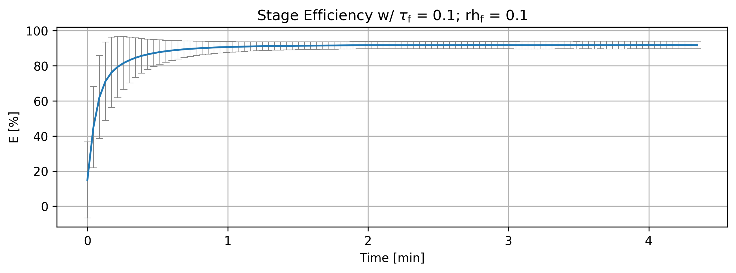
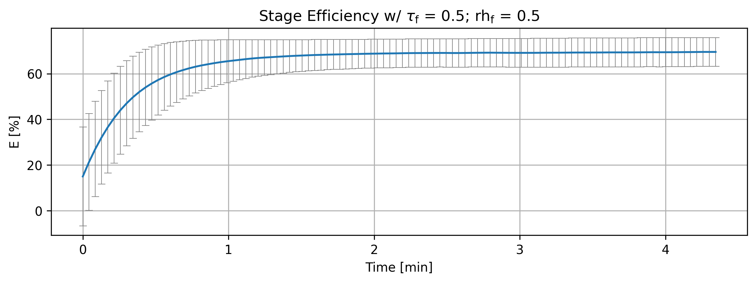
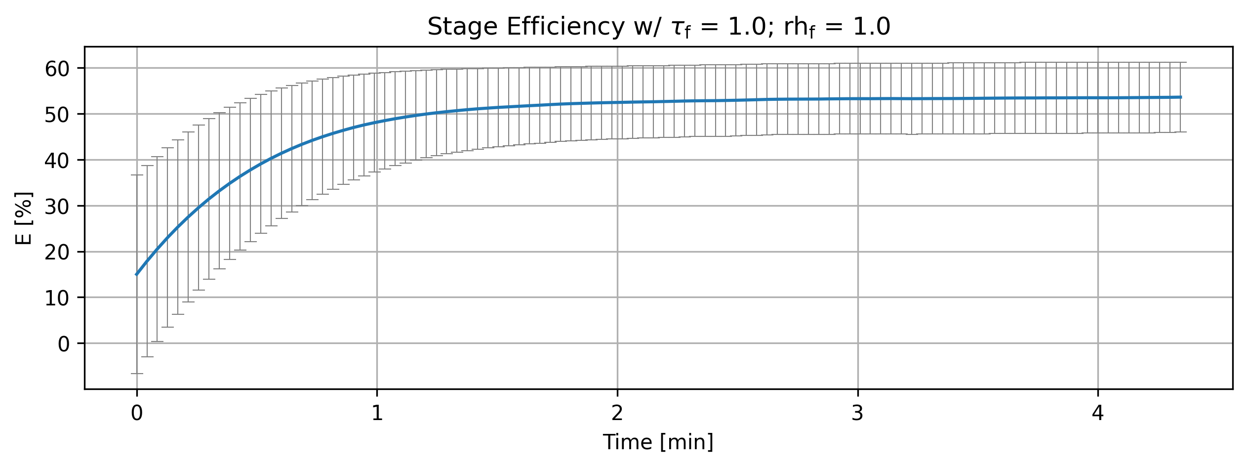
quant.plot(title=r'Stage Efficiency w/ $\tau_{\mathrm{f}}$ = %2.1f; rh$_{\mathrm{f}}$ = %2.1f'%(tau,rh), x_scaling=1/unit.min, x_label='Time [min]', y_label=quant.latex_name+
' ['+quant.unit+']', show=True, figsize=[10,3], error_data=True, error_fill=False)
if cortix_ai:
cortix_ai.explain(markdown_display=markdown_display, save_supporting_info=db_save)
fig_count += 1
print(f'Figure {fig_count}: Stage efficiency variation with parameters.')
Cortix AI assistant: working on explanation...
Overview
The script builds and plots per-stage efficiency histories for a sequence of stage objects, annotating each plotted quantity with parameter values and incrementing a figure counter before printing a summary line.
Imports and setup
from cortix import Units as unit: imports unit definitions; unit.min is later used for x-axis scaling.
import matplotlib.pyplot as plt: standard plotting library (plt is not used directly in the shown snippet but is available).
efficiencies = list(): prepares an empty list to accumulate efficiency-history objects.
Collection of efficiency histories
for stg in stages: iterates over an iterable named stages (each element expected to be a stage object).
stg.efficiency_history(mean=True) is called for each stage; the returned object is appended to efficiencies.
The appended objects (referred to later as eff) represent time-series quantities with metadata (name, value, unit, latex_name, and plotting methods).
Per-parameter plotting loop
for eff, tau, rh in zip(efficiencies, param_tau_factors, param_inflow_rh_factors): iterates in parallel over the collected efficiency objects and two parameter lists (tau factors and relative-humidity factors).
quant = eff: assigns a local reference quant to the current efficiency object.
quant.name += f”””; @ parameter tau factor = {tau} and parameter relative humidity {rh}”””: appends parameter information to the quantity’s name string.
quant.value.name = quant.name: sets the nested value name to match the updated quantity name (so associated value metadata carries the same label).
quant.plot(…): calls the quantity’s plot method with these arguments:
title: a raw string containing LaTeX fragments and then formatted with %2.1f for tau and rh (so the title shows numeric values with one decimal place). Example pattern: Stage Efficiency w/ $\tau_{\mathrm{f}}$ = 1.0; rh$_{\mathrm{f}}$ = 0.5
x_scaling=1/unit.min: rescales the time axis from base units to minutes (factor 1 per minute).
x_label=’Time [min]’: label for the x axis.
y_label=quant.latex_name + ‘ [’ + quant.unit + ‘]’: constructs the y-axis label from the quantity’s LaTeX name and its unit in square brackets.
show=True: display the plot immediately (handled by the quantity’s plot method).
figsize=[10,3]: figure size in inches (wide and short).
error_data=True, error_fill=False: request plotting of error bars/data but disable a filled error band (specific rendering governed by the plot implementation).
Conditional auxiliary call and final output
if cortix_ai: cortix_ai.explain(markdown_display=markdown_display, save_supporting_info=db_save)
The call to cortix_ai.explain is executed only if cortix_ai evaluates truthy; it is invoked with two keyword arguments passed through from local variables.
fig_count += 1: increments a running figure counter (assumes fig_count was defined earlier).
print(f’Figure {fig_count}: Stage efficiency variation with parameters.’): prints a one-line summary identifying the updated figure count and the plotted content.
Data and side-effect summary
Side effects performed by the snippet:
Mutates quantity metadata (quant.name and quant.value.name) to include parameter annotations.
Produces one plot per zipped tuple (efficiency, tau, rh) via quant.plot.
Optionally calls cortix_ai.explain when cortix_ai is present.
Increments and prints fig_count.
Inputs expected (not defined in snippet):
stages: iterable of stage objects exposing efficiency_history(mean=True).
param_tau_factors and param_inflow_rh_factors: iterables of numeric parameter values of equal length to efficiencies.
cortix_ai, markdown_display, db_save, fig_count: external variables referenced by the snippet.
AI Parameters:
+ LLM model (OpenAI) = gpt-5-mini
+ LLM cleverness = 1.0
+ Total # of tokens = 3753
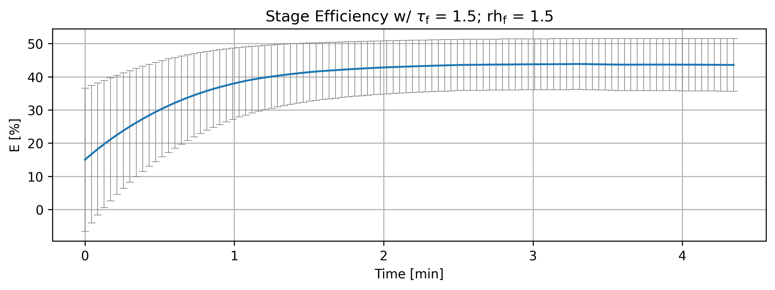
Figure 1: Stage efficiency variation with parameters.
1.3.1. Analysis#
LLM analysis.
'''Analyze efficiencies'''
if cortix_ai:
    cortix_ai.explain(quant=efficiencies, markdown_header_level='<h4>', markdown_display=markdown_display, save_supporting_info=db_save)
Cortix AI assistant: working on explanation...
Summary
Four time-series (tau factor = 0.1, 0.5, 1.0, 1.5) share the same time grid (0 … 247.699 s) and identical initial values at t = 0 (column 0 = 15.0002, column 1 = 21.6026).
Column “0” increases with time and approaches a plateau; column “1” decreases with time and approaches a low steady value.
The rate and asymptotic values depend strongly on the tau factor: smaller tau → faster rise of column 0 and faster fall of column 1.
Time evolution — column 0 (first numeric column)
At t = 0 all cases start at 15.0002.
Early-time growth (t ≈ 15–31 s) is much faster for small tau:
tau = 0.1: 81.53 (t = 15.48 s) → 87.78 (t = 30.96 s)
tau = 0.5: 44.03 → 57.24
tau = 1.0: 29.54 → 39.04
tau = 1.5: 23.79 → 30.37
Long-time plateau (t = 247.699 s) values:
tau = 0.1: 91.7701
tau = 0.5: 69.4544
tau = 1.0: 53.4794
tau = 1.5: 43.6286
Interpretation: increasing tau factor slows the approach to higher efficiency and lowers the asymptotic efficiency in column 0.
Time evolution — column 1 (second numeric column)
All cases start at 21.6026 and monotonically decrease.
Early-time decrease (t ≈ 15–31 s):
tau = 0.1: 21.60 → 15.09 → 6.91 by 30.96 s
tau = 0.5: 21.60 → 19.21 → 15.29
tau = 1.0: 21.60 → 17.99 → 15.15
tau = 1.5: 21.60 → 17.37 → 14.53
Long-time plateau (t = 247.699 s) values:
tau = 0.1: 2.12651
tau = 0.5: 6.34104
tau = 1.0: 7.69490
tau = 1.5: 7.90588
Interpretation: smaller tau yields a faster and deeper reduction in column 1; larger tau produces a slower decline and a higher steady residual.
Direct comparison and key takeaways
At intermediate and long times, the series are well separated by tau:
Column 0 ordering (largest to smallest) at t = 247.7 s: tau 0.1 > 0.5 > 1.0 > 1.5.
Column 1 ordering (smallest to largest) at t = 247.7 s: tau 0.1 < 0.5 < 1.0 < 1.5.
Magnitude of change relative to t = 0:
Column 0 net increase by t = 247.7 s:
+76.77 (tau 0.1), +54.45 (0.5), +38.48 (1.0), +28.63 (1.5).
Column 1 net decrease by t = 247.7 s:
−19.48 (tau 0.1), −15.26 (0.5), −13.91 (1.0), −13.70 (1.5).
Dynamics:
tau = 0.1 reaches near-steady values earlier (by ~30–120 s) compared with larger tau where approach to steady state is slower and plateaus at lower (column 0) / higher (column 1) magnitudes.
Overall conclusion: Tau factor is a controlling time-scale parameter here — smaller tau accelerates conversion of the quantity represented by column 1 into that represented by column 0 and produces a higher steady-state for column 0 and a lower residual for column 1.
AI Parameters:
+ LLM model (OpenAI) = gpt-5-mini
+ LLM cleverness     = 1.0
+ Total # of tokens  = 5879
'''Stage overall efficiency'''
from cortix import Units as unit
import matplotlib.pyplot as plt

for eff, tau, rh in zip(efficiencies, param_tau_factors, param_inflow_rh_factors):
    quant = eff
    quant.plot(title=r'Stage Efficiency w/ $\tau_\mathrm{f}$ = %2.1f; rh$_{\mathrm{f}}$ = %2.1f'%(tau,rh), x_scaling=1/unit.min, x_label='Time [min]', y_label=quant.latex_name+
               ' ['+quant.unit+']', legend=['E', 'std'], show=True, figsize=[10,3], error_data=False, error_fill=False)
fig_count += 1
print(f'Figure {fig_count}: Stage efficiency and deviation variation with parameters.')
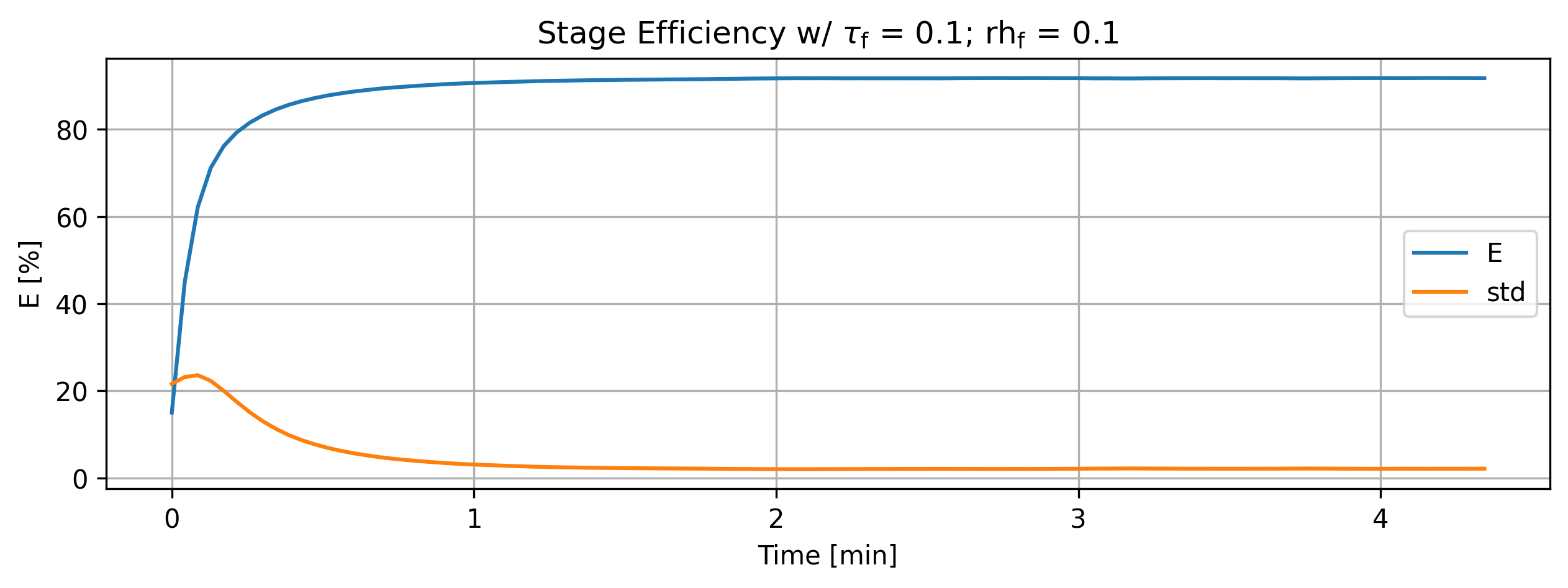
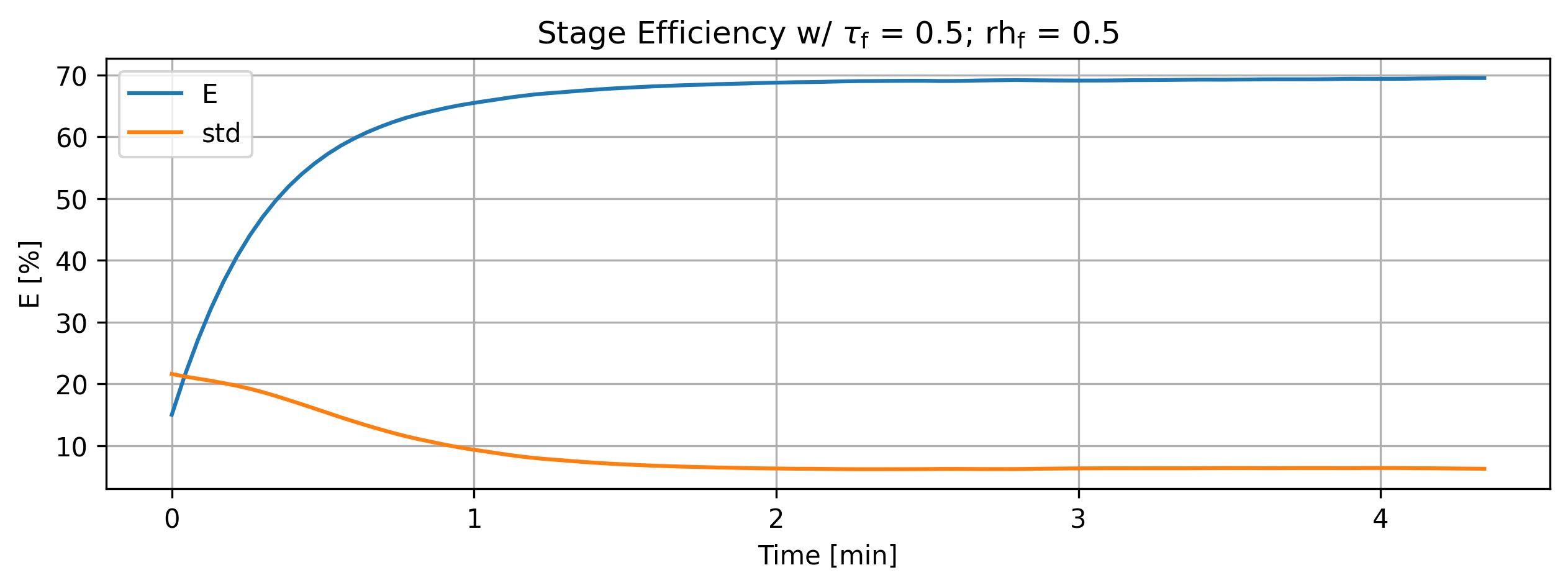
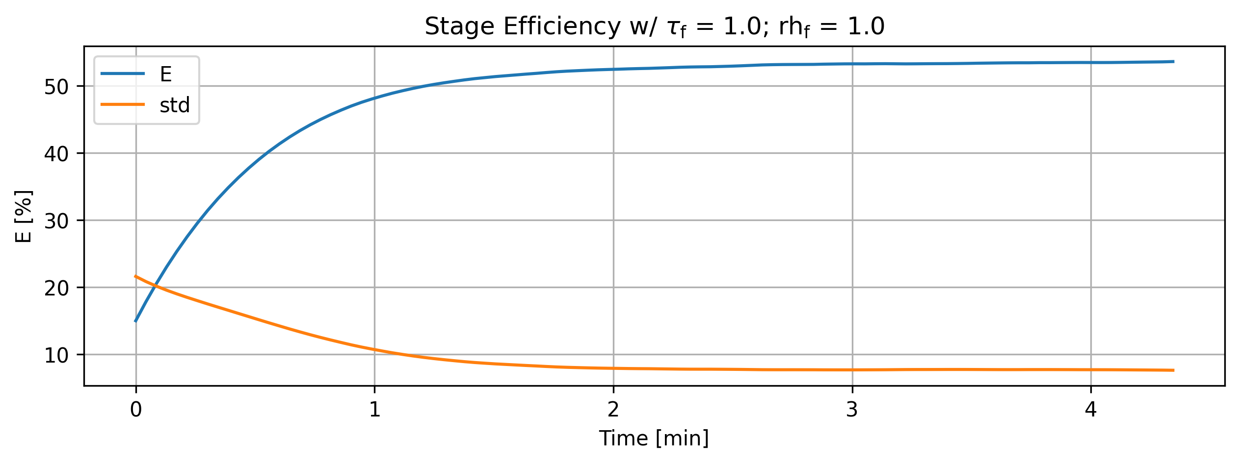
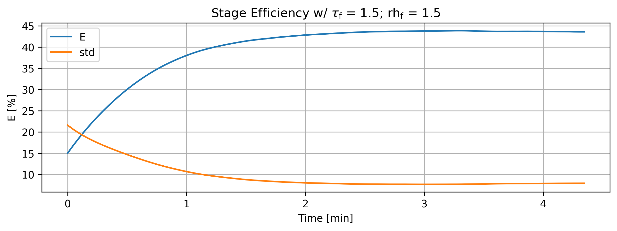
Figure 2: Stage efficiency and deviation variation with parameters.
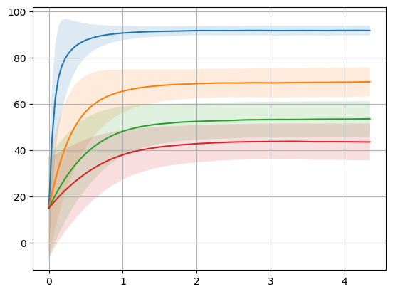
'''For debugging purposes'''
import matplotlib.pyplot as plt
import numpy as np

for eff in efficiencies:
    data = eff.value
    values = list()
    errors = list()
    for entry in data:
        values.append(entry[0])
        errors.append(entry[1])
    values = np.array(values)
    errors = np.array(errors)

    plt.plot(data.index/60, values)
    plt.fill_between(data.index/60, values - errors, values + errors, alpha=0.15)

plt.grid()

fig_count += 1
print(f'Figure {fig_count}: Multiplot efficiency variation with parameters.')
Figure 3: Multiplot efficiency variation with parameters.