Single-Stage Solvex Development Cortix Tech 30Sep2025

1. Use-Case 02: TBP-Diluent-H\(_2\)O-Air Mixing

Developer: Valmor F. de Almeida, PhD

Cortix Tech, Lowell, MA 01854, USA

Revision date: 02Dec25

1.1. Objectives

• Develop usecase scenario for water extraction by TBP with a vapor phase.

• Test implementation and present results.

• Use AI assistants to help with information and reporting.

  • AI requests below may need to be executed multiple times if the result is not satisfactory or incorrect.

'''AI assistance options'''
# Set all to False if you do not have access to OpenAI API and/or AI codes below
cortix_ai = True
stage_ai = True

'''Generate proprietary knowledge database?'''
db_save = False # set this to false if going public (online) with this notebook

'''Other helpers'''
fig_count = 0
tbl_count = 0
markdown_display = True # if False code cell output is type: stream, else: markdown. Use True for in-house conversion to .md

1.2. System

Single stage mixing of air, water, and TBP with inert diluent.

'''Setup the base system'''
from cortix import Cortix
from cortix import Network
from cortix import Units as unit
from cortix import ReactionMechanism
from cortix import Quantity

system = Cortix(use_mpi=False, splash=True) # System top level
system_net = system.network = Network() # Network

if cortix_ai:
    from cortix import CortixAI
    cortix_ai = CortixAI(llm_model='gpt-5-mini', llm_cleverness=0.8)
    cortix_ai.markdown_header_level = '<h3>'
    cortix_ai.n_chunks = 8

if cortix_ai: 
    cortix_ai.explain(markdown_display=markdown_display, print_prompt=False, save_supporting_info=db_save)

[31384] 2025-12-02 15:40:12,335 - cortix - INFO - Created Cortix object 
_____________________________________________________________________________
                             L A U N C H I N G                               
_____________________________________________________________________________
      ...                                        s       .     (TAAG Fraktur)
   xH88"`~ .x8X                                 :8      @88>
 :8888   .f"8888Hf        u.      .u    .      .88      %8P      uL   ..
:8888>  X8L  ^""`   ...ue888b   .d88B :@8c    :888ooo    .     .@88b  @88R
X8888  X888h        888R Y888r ="8888f8888r -*8888888  .@88u  ""Y888k/"*P
88888  !88888.      888R I888>   4888>"88"    8888    888E`    Y888L
88888   %88888      888R I888>   4888> "      8888      888E      8888
88888 `> `8888>     888R I888>   4888>        8888      888E      `888N
`8888L %  ?888   ! u8888cJ888   .d888L .+    .8888Lu=   888E   .u./"888&
 `8888  `-*""   /   "*888*P"    ^"8888*"     ^%888*     888&  d888" Y888*"
   "888.      :"      "Y"          "Y"         "Y"      R888" ` "Y   Y"
     `""***~"`                                           ""
                             https://cortix.org                              
_____________________________________________________________________________
Cortix AI assistant: working on explanation...

Overview

• This snippet sets up a Cortix simulation object, attaches a network, conditionally constructs a CortixAI helper, configures a few of its attributes, and (conditionally) calls its explain method with three arguments.

Imports

• from cortix import Cortix

• from cortix import Network

• from cortix import Units as unit

• from cortix import ReactionMechanism

• from cortix import Quantity

  • These imports bring top-level Cortix classes and utilities into the local namespace. In this snippet, Cortix and Network are used directly; Units (aliased unit), ReactionMechanism, and Quantity are imported but not referenced further.

System and network initialization

• system = Cortix(use_mpi=False, splash=True)

  • Instantiates the top-level Cortix object named system.

  • Keyword use_mpi=False requests a non-MPI (single-process) instantiation.

  • Keyword splash=True requests the library’s startup banner or splash behavior.

• system_net = system.network = Network()

  • Creates a new Network() instance.

  • Assigns that instance to the attribute system.network and also to the local variable system_net, so both reference the same Network object.

Conditional CortixAI creation and configuration

• if cortix_ai:

  • The block executes only if the name cortix_ai exists in the current scope and evaluates as truthy.

  • Inside the block:

    • from cortix import CortixAI

      • Lazily imports CortixAI (only when the condition is true).

    • cortix_ai = CortixAI(llm_model=’gpt-5-mini’, llm_cleverness=0.8)

      • Reassigns the name cortix_ai to a newly created CortixAI instance configured with an LLM model identifier and a “cleverness” parameter.

    • cortix_ai.markdown_header_level = ‘

      ’

      • Sets an attribute on the CortixAI instance that controls the markdown header level it will use.

    • cortix_ai.n_chunks = 8

      • Sets an attribute that likely controls chunking behavior (number of chunks) on the CortixAI instance.

Second conditional and explain invocation

• if cortix_ai:

  • If cortix_ai is truthy in the current scope, this block calls:

    • cortix_ai.explain(markdown_display=markdown_display, print_prompt=False, save_supporting_info=db_save)

      • The explain method is invoked with three keyword arguments:

        • markdown_display (a variable expected to exist in scope),

        • print_prompt set to False,

        • save_supporting_info set to the value of db_save (also expected to exist in scope).

      • No description of the method’s behavior is provided here (the snippet calls it but its internal effect is not detailed).

Runtime and name-resolution notes

• The conditionals use the name cortix_ai before it is assigned within the first block; therefore, at runtime:

  • If cortix_ai is not defined earlier in the surrounding scope, evaluating if cortix_ai will raise a NameError.

  • If cortix_ai is defined and truthy, the first block will reassign cortix_ai to a CortixAI instance; otherwise neither block runs.

• The variables markdown_display and db_save used in the final call must also be defined elsewhere in scope for that call to succeed.

AI Parameters:
+ LLM model (OpenAI) = gpt-5-mini
+ LLM cleverness     = 1.0
+ Total # of tokens  = 3594

'''FYI LLM models info'''
if cortix_ai:
    print(cortix_ai.llm_names_info)

{'gpt-5': 'Full reasoning-intensive tasks', 'gpt-5-mini': 'Balance of speed and capability', 'gpt-5-nano': 'Speed and cost efficiency', 'gpt-4o-mini': 'Fastest at advanced reasoning', 'gpt-4o': 'Great for most tasks', 'gpt-4.1': 'Great for quick coding and analysis', 'gpt-4.1-mini': 'Faster than 4.1 for everyday tasks'}

1.2.1. Stage

Instantiate a single stage to model and simulate the reactive mixing process.

'''Import Stage'''
from solvex import Stage

'''Create and Configure a StageAI Object'''
if stage_ai:
    from stage_ai import StageAI
    stage_ai = StageAI(llm_model='gpt-5-mini', llm_cleverness=0.8)
    stage_ai.markdown_header_level = '<h4>'

if stage_ai:
    stage_ai.help('stage', markdown_display=markdown_display, print_prompt=False, save_supporting_info=db_save)

Stage AI assistant: working on help...

Stage Description

Overview

This document summarizes the main design, dataflow and runtime behaviour of the Stage module (solvent-extraction stage) implemented in stage.py. The Stage models three co-existing phases, reaction-driven species generation/consumption, and transport through inflow/outflow ports. It integrates a reaction mechanism, time-integrates mass balances, records phase histories and exposes history/diagnostic quantities.

Below is the original stage schematics (copied verbatim from the module docstring):

                         Aqueous    Organic
                        External    Product
                          Feed
                            |          ^
                            |          |
                            |          |
                            V          |
                       |---------------------|
  Vapor/Org inter-stage|                     | Vapor/Aqu inter-stage
  outflow <------------|                     |-----------> outflow
                       |                     |
  Organic inter-stage  |    S O L V E N T    | Aqueous inter-stage
  outflow <------------| E X T R A C T I O N |-----------> outflow
                       |                     |
                       |                     |
  Vapor/Aqu inter-stage|      S T A G E      | Vapor/Org inter-stage
  inflow  ------------>|                     |<----------- inflow
                       |                     |
  Aqueous inter-stage  |                     | Organic inter-stage
  inflow ------------->|                     |<----------- inflow
                       |---------------------|
                            |          ^
                            |          |
                            |          |
                            V          |
                         Aqueous    Organic
                         Product    External
                                      Feed

Phases involved

• The Stage explicitly manages three phase containers: aqueous phase, organic phase, and vapor phase.

• Each phase is represented by a Phase (PhaseNew) object and holds species concentrations and a time-indexed history (rows are time-stamped).

Note: information about a stage module is needed: stage

Module structure and key components

• Class: Stage(Module)

  • Purpose: represent a single solvent-extraction contactor stage with mixing volume, flows and reactions.

  • High-level responsibilities:

    1. Hold phase containers and inflow-parameter containers.

    2. Accept a ReactionMechanism and map species into phase-local lists.

    3. Assemble a global state vector for ODE integration.

    4. Integrate the mass-balance ODEs over time steps with scipy.odeint.

    5. Provide diagnostics and time histories (reaction rates, generation rates, efficiencies, mass-density, etc.).

• Phases and inflows:

  • For each physical phase (aqueous, organic, vapor) there is a phase container created by methods:

    • __setup_aqueous_phase()

    • __setup_organic_phase()

    • __setup_vapor_phase()

  • For inflow parameter storage there are separate Phase containers created with names such as ‘inflow-aqueous’, ‘inflow-organic’, etc.

Important attributes

• mix_vol: mixing volume for the stage (SI units).

• vol_flowrate_org, vol_flowrate_aqu, vol_flowrate_vap_org, vol_flowrate_vap_aqu: configured volumetric flowrates.

• volume_fractions: dictionary with phase volume fractions {‘(o)’:…, ‘(a)’:…, ‘(v)’:…}.

• rxn_mech: ReactionMechanism instance assigned via add_reaction_mechanism(…).

• phase containers: self.aqueous_phase, self.organic_phase, self.vapor_phase.

• inflow containers: self.inflow_aqueous_phase, self.inflow_organic_phase, self.inflow_vapor_aqueous_phase, self.inflow_vapor_organic_phase.

• ode solver parameters: self.__ode_params (contains temperature etc.).

Ports (existence and single-line listing)

• The Stage exposes multiple ports for connecting inflows and outflows (feeds, products and inter-stage links). These ports are declared in self.port_names_expected when the Stage is constructed.

ports = [‘aqu-feed’,’org-feed’,’aqu-product’,’org-product’,’aqu-inflow’,’org-inflow’,’aqu-outflow’,’org-outflow’,’vap-aqu-inflow’,’vap-org-inflow’,’vap-aqu-outflow’,’vap-org-outflow’]

Key methods (signatures only)

• init(self, mix_vol, vol_flowrates, temperature)

• add_reaction_mechanism(self, rxn_mech=None)

• run(self, *args)

• __call_ports(self, time)

• __step(self, time=0.0)

• __get_state_vector(self, time=None, cc_name=’mass_cc’)

• __mbal_rhs_func(self, u_vec, time, params)

• __update_outflow_mass_rates(self, u_vec)

• __convert_mass_cc_to_molar_cc(self, u_vec)

• __update_state_variables(self, u_vec, time)

• r_vec(self, time=None)

• g_vec(self, time=None)

• rxn_efficiencies(self, time=None)

• efficiency_history(self, rxn_id=None, mean=False)

• mass_density_history(self, phase_name=None)

• mass_balance_residual_history(self)

Brief code snippet: example of key class method signatures

class Stage(Module):
    def __init__(self, mix_vol, vol_flowrates, temperature):
        ...

    def add_reaction_mechanism(self, rxn_mech=None):
        ...

    def run(self, *args):
        ...

    def __step(self, time=0.0):
        ...

    def __mbal_rhs_func(self, u_vec, time, params):
        ...

The step method (what it does) and example snippet

• Purpose: advance the internal stage state forward by one configured time_step.

• Main actions performed in each step:

  1. Build current state vector from phase containers (__get_state_vector).

  2. Integrate the mass-balance ODE system over [time, time + time_step] using odeint and the RHS function __mbal_rhs_func.

  3. Validate solver success and check mass conservation (optionally printing residuals).

  4. Optionally compute and print total mass inflow/outflow rates.

  5. Update all phase containers with the solution at the new time (via __update_state_variables).

• Short representative snippet (extracted and condensed for clarity):

def __step(self, time=0.0):
    u_vec_0 = self.__get_state_vector(time)
    t_interval = np.linspace(time, time+self.time_step, num=2)

    (u_vec_hist, info_dict) = odeint(self.__mbal_rhs_func,
                                     u_vec_0, t_interval,
                                     args=(self.__ode_params,),
                                     full_output=True)

    assert info_dict['message'] == 'Integration successful.'
    u_vec = u_vec_hist[1,:]
    time += self.time_step

    # mass-conservation checks, diagnostics, then update phase containers
    self.__update_state_variables(u_vec, time)
    return time

mass-balance RHS function (role and signature)

• Signature: __mbal_rhs_func(self, u_vec, time, params)

• Role: compute dt_u (time derivatives of the global state vector) to be consumed by the ODE integrator. It:

  • Enforces non-negativity on u_vec (clips negatives to zero).

  • Updates state-derived outflow mass rates from u_vec (__update_outflow_mass_rates).

  • Converts mass concentrations to molar concentrations (per phasic-volume basis) for reaction computations (__convert_mass_cc_to_molar_cc).

  • Calls the reaction mechanism to obtain species generation rates per mixing-volume (g_vec = rxn_mech.g_vec(…)).

  • Assembles dt_u for each phase by combining inflow/outflow mass flow rates, reaction generation (converted to mass units via molar mass) and dividing by phase volume fraction (phi).

  • Returns dt_u as a numpy array of length = total number of species in rxn_mech.

Ports usage and call ports in time stepping

• Ports are used to exchange mass-flowrate vectors and timestamps with neighbouring stages/modules.

• __call_ports(time) is invoked after every successful __step to:

  • Send/receive data on inflow ports (e.g. ‘aqu-inflow’) and update inflow parameter containers if connected.

  • Receive outflow requests and respond when this Stage is a supplier.

• Typical port usage pattern in run():

  1. Before stepping, __update_mass_inflow_rates() collects parameter inflow mass rates from inflow Phase containers (or from connected ports if present).

  2. At each time-step iteration in run(), Stage perturbs inflow rates if requested, calls __step(), then __call_ports(time) to exchange current mass-rate data with connected neighbours.

• The port API used by Stage includes send() and recv() helpers (inherited from Module). The logic in __call_ports ensures consistency checks (time match) and that received mass-rate arrays have the expected length.

Time stepping and run()

• run(self, *args) is the driving loop that:

  • Rebuilds logger, ensures end_time is at least initial_time + time_step.

  • Calls __update_mass_inflow_rates() at start to pick up parameter inflows.

  • Enters a while loop advancing time until end_time:

    • Optionally log progress.

    • Optionally perturb inflow rates (__perturb_mass_inflow_rates).

    • Call __step(time) to integrate one time_step.

    • Call __call_ports(time) to exchange mass-rate data.

  • After finishing, final summary logging is performed if requested.

Data history and diagnostics

• Each phase is a time-stamped table: phase.add_row(time, values) records mass concentrations for species.

• Utility methods exposed include:

  • r_vec(time=None): instantaneous reaction rate density vector (mol/vol/time).

  • g_vec(time=None): instantaneous species generation rate density vector (mol species/vol/time).

  • rxn_efficiencies(time=None): computes per-reaction conversion efficiencies (useful for heterogeneous reactions with mass transfer).

  • r_vec_history, g_vec_history, efficiency_history, mass_density_history, mass_balance_residual_history: assemble pandas Series wrapped in Quantity objects for plotting/analysis.

Usage notes for code users

• Typical workflow:

  1. Instantiate Stage(mix_vol, vol_flowrates, temperature).

  2. Create and add a ReactionMechanism via add_reaction_mechanism(…). This sets up all species and global ids used in state vectors.

  3. Optionally seed inflow Phase containers (inflow_aqueous_phase, inflow_organic_phase, … ) with species concentrations (these are parameters used to compute mass inflow rates).

  4. Configure simulation timing (initial_time, end_time, time_step) and logging verbosity.

  5. Connect ports if composing multiple Stage modules; otherwise the Stage will use local inflow parameter containers.

  6. Call run(…) with appropriate context (in the example, run receives args whose first item is a logger-like object containing a name).

• When connecting modules: ensure connected ports exchange a (time, mass_rates_array) tuple where the mass_rates array matches the expected species count for the phase.

Summary

• Stage is a compact, phase-aware transient mass-balance solver for a solvent-extraction mixing stage. It separates phases into independent containers, maintains inflow parameter containers, integrates a global mass-balance ODE assembled from phase-local species, and exchanges mass-rate information via ports. The two critical pieces for extension or integration are the reaction mechanism (ReactionMechanism) and correct wiring of ports when composing multiple stages.

AI Parameters:
+ LLM model (OpenAI) = gpt-5-mini
+ LLM cleverness     = 1.0
+ RAG                = stage.py
+ Total # of tokens  = 18726
Done with help...

'''FYI LLM models info'''
if stage_ai:
    print(stage_ai.llm_names_info)

{'gpt-5': 'Full reasoning-intensive tasks', 'gpt-5-mini': 'Balance of speed and capability', 'gpt-5-nano': 'Speed and cost efficiency', 'gpt-4o-mini': 'Fastest at advanced reasoning', 'gpt-4o': 'Great for most tasks', 'gpt-4.1': 'Great for quick coding and analysis', 'gpt-4.1-mini': 'Faster than 4.1 for everyday tasks'}

1.2.1.1. Configuration

'''Create Stage and add system'''
from solvex import Stage

# Initialization
mixing_volume = 1*unit.L
# Aqueous phase
mixing_vol_flowrate_aqu = 500*unit.mL/unit.min
# Organic phase
mixing_vol_flowrate_org = 600*unit.mL/unit.min
# Vapor phase
mixing_vol_flowrate_vap = (3.7*mixing_vol_flowrate_org/100, 8.1*mixing_vol_flowrate_aqu/100) # percentage of (org, aqu)

mixing_vol_flowrates = [mixing_vol_flowrate_org, mixing_vol_flowrate_aqu, mixing_vol_flowrate_vap]

stg_temperature = unit.convert_temperature(40, 'C', 'K')

stg = Stage(mixing_volume, mixing_vol_flowrates, stg_temperature) # Create solvent extraction module

system_net.module(stg)

if cortix_ai:
    cortix_ai.explain(markdown_header_level='<h5>', markdown_display=markdown_display, save_supporting_info=db_save)

Cortix AI assistant: working on explanation...

Overview

• The snippet constructs a solvent-extraction Stage object with specified mixing volume, phase flowrates, and temperature, then attaches it to a system network and conditionally invokes a Cortix AI helper.

Imports and intent

• from solvex import Stage: the code uses the Stage class from the solvex package to represent a solvent-extraction module (a unit operation that mixes phases).

Configured quantities (variables and units)

• mixing_volume: a volume value set to 1 L (using a units-aware quantity, e.g., unit.L).

• mixing_vol_flowrate_aqu: aqueous-phase volumetric flowrate set to 500 mL/min.

• mixing_vol_flowrate_org: organic-phase volumetric flowrate set to 600 mL/min.

• mixing_vol_flowrate_vap: a tuple of two values computed as percentages of the org and aqu flowrates:

  • first element: 3.7% of the organic flowrate (3.7 * mixing_vol_flowrate_org / 100).

  • second element: 8.1% of the aqueous flowrate (8.1 * mixing_vol_flowrate_aqu / 100).

• mixing_vol_flowrates: a list bundling the phase flowrates in the order [organic, aqueous, vapor].

• stg_temperature: the stage temperature obtained by converting 40 °C to Kelvin using unit.convert_temperature(40, ‘C’, ‘K’).

Stage creation and system integration

• stg = Stage(mixing_volume, mixing_vol_flowrates, stg_temperature):

  • Instantiates a Stage object with the given total mixing volume, the list of per-phase volumetric flowrates, and the temperature in Kelvin.

  • The Stage likely encapsulates behavior and state for a solvent-extraction stage (mass/volume balance and mixing), as represented by the solvex Stage class.

• system_net.module(stg):

  • Adds the created Stage instance to the system network object system_net (registers the module within the larger process/network model).

Conditional Cortix AI call

• if cortix_ai:

  • The code checks whether a cortix_ai object/reference is truthy; if so, it calls cortix_ai.explain(…) with parameters markdown_header_level=’

    ’, markdown_display=markdown_display, save_supporting_info=db_save.

  • No further description of the explain() implementation is provided here.

Type and evaluation notes

• Numeric operations combine unit-bearing quantities; e.g., multiplying a unit-aware flowrate by a scalar and dividing by 100 yields another quantity with the same flowrate units.

• The vapor flowrates are provided as a tuple of two computed quantities (percent-based contributions), then placed into the list with the other flowrates, so the Stage receives a mixed-type iterable of per-phase flowrate quantities.

• Order matters: the flowrates list is explicitly [org, aqu, vap], so the Stage will interpret the first element as organic flow, second as aqueous, third as vapor.

AI Parameters:
+ LLM model (OpenAI) = gpt-5-mini
+ LLM cleverness     = 1.0
+ Total # of tokens  = 3372

print('Flow residence time [s]: average = %5.3e'%stg.flow_residence_time_avg)
print('Aqueous volume fraction = %5.3e'%stg.volume_frac_aqu) 
print('Organic volume fraction = %5.3e'%stg.volume_frac_org) 
print('Vapor volume fraction   = %5.3e'%stg.volume_frac_vap) 

Flow residence time [s]: average = 5.160e+01
Aqueous volume fraction = 4.300e-01
Organic volume fraction = 5.160e-01
Vapor volume fraction   = 5.393e-02

'''Draw the Cortix network system'''
system_net.draw(engine='circo', node_shape='folder', ports=True)

'''For help purposes'''
import solvex.stage

Documentation options:

• Live in this notebook run on code cell: help(solvex_ustc.stage)

• On the web: source

# Poor's man help
#help(solvex_ustc.stage)

1.2.2. Reaction Mechanism

Contacting water, inert diluent and TBP, and air.

1.2.2.1. Water extraction example

args_dict = {'water_activity': 1.0}
file_name = 'tbp-h2o-air.txt'
rxn_mech = ReactionMechanism(file_name=file_name, order_species=True, args_dict=args_dict)

WARNING: ReactionMechanism: user must implement a H2O*[C4H9O]3PO(o) product partition function with signature <product>(rxn_mech, temperature, spc_molar_cc, arg_dict) function for [C4H9O]3PO(o) + H2O(a) <-> H2O*[C4H9O]3PO(o) 
WARNING: ReactionMechanism: user must implement a [H2O]2*[[C4H9O]3PO]2(o) product partition function with signature <product>(rxn_mech, temperature, spc_molar_cc, arg_dict) function for 2 [C4H9O]3PO(o) + 2 H2O(a) <-> [H2O]2*[[C4H9O]3PO]2(o) 
WARNING: ReactionMechanism: user must implement a [H2O]6*[[C4H9O]3PO]3(o) product partition function with signature <product>(rxn_mech, temperature, spc_molar_cc, arg_dict) function for 3 [C4H9O]3PO(o) + 6 H2O(a) <-> [H2O]6*[[C4H9O]3PO]3(o) 
WARNING: ReactionMechanism: user must implement a H2O(v) product partition function with signature <product>(rxn_mech, temperature, spc_molar_cc, arg_dict) function for H2O(a) <-> H2O(v) 
WARNING: ReactionMechanism: user must implement a O2(a) product partition function with signature <product>(rxn_mech, temperature, spc_molar_cc, arg_dict) function for O2(v) <-> O2(a)   
WARNING: ReactionMechanism: user must implement a N2(a) product partition function with signature <product>(rxn_mech, temperature, spc_molar_cc, arg_dict) function for N2(v) <-> N2(a)   

#'''User input'''
#rxn_mech.cat_input()

#'''Show Mechanism'''
# Jupyter Book does not render LaTeX through IPython.display(Markdown)
#rxn_mech.md_print()

#'''Species and reactions manual output'''
#print(len(rxn_mech.species_names), ' **Species**\n', rxn_mech.latex_species)
#print(len(rxn_mech.reactions), ' **Reactions**\n', rxn_mech.latex_rxn)

10 Species

\[\begin{align*} &{\mathrm{H}_{2}\mathrm{O}}_\mathrm{(a)}, {\mathrm{H}_{2}\mathrm{O}}_\mathrm{(v)}, {\mathrm{H}_{2}\mathrm{O}\bullet[\mathrm{C}_{4}\mathrm{H}_{9}\mathrm{O}]_{3}\mathrm{P}\mathrm{O}}_\mathrm{(o)}, {\mathrm{N}_{2}}_{\mathrm{(a)}}, {\mathrm{N}_{2}}_{\mathrm{(v)}}, {\mathrm{O}_{2}}_{\mathrm{(a)}}, {\mathrm{O}_{2}}_{\mathrm{(v)}}, {[\mathrm{C}_{4}\mathrm{H}_{9}\mathrm{O}]_{3}\mathrm{P}\mathrm{O}}_\mathrm{(o)}, \\ & {[\mathrm{H}_{2}\mathrm{O}]_{2}\bullet[[\mathrm{C}_{4}\mathrm{H}_{9}\mathrm{O}]_{3}\mathrm{P}\mathrm{O}]_{2}}_{\mathrm{(o)}}, {[\mathrm{H}_{2}\mathrm{O}]_{6}\bullet[[\mathrm{C}_{4}\mathrm{H}_{9}\mathrm{O}]_{3}\mathrm{P}\mathrm{O}]_{3}}_{\mathrm{(o)}}\end{align*}\]

6 Reactions

\[\begin{align*} {\mathrm{H}_{2}\mathrm{O}}_\mathrm{(a)}\ + \ {[\mathrm{C}_{4}\mathrm{H}_{9}\mathrm{O}]_{3}\mathrm{P}\mathrm{O}}_\mathrm{(o)}\ &\longleftrightarrow \ {\mathrm{H}_{2}\mathrm{O}\bullet[\mathrm{C}_{4}\mathrm{H}_{9}\mathrm{O}]_{3}\mathrm{P}\mathrm{O}}_\mathrm{(o)}\\ 2.0\,{\mathrm{H}_{2}\mathrm{O}}_\mathrm{(a)}\ + \ 2.0\,{[\mathrm{C}_{4}\mathrm{H}_{9}\mathrm{O}]_{3}\mathrm{P}\mathrm{O}}_\mathrm{(o)}\ &\longleftrightarrow \ {[\mathrm{H}_{2}\mathrm{O}]_{2}\bullet[[\mathrm{C}_{4}\mathrm{H}_{9}\mathrm{O}]_{3}\mathrm{P}\mathrm{O}]_{2}}_{\mathrm{(o)}}\\ 6.0\,{\mathrm{H}_{2}\mathrm{O}}_\mathrm{(a)}\ + \ 3.0\,{[\mathrm{C}_{4}\mathrm{H}_{9}\mathrm{O}]_{3}\mathrm{P}\mathrm{O}}_\mathrm{(o)}\ &\longleftrightarrow \ {[\mathrm{H}_{2}\mathrm{O}]_{6}\bullet[[\mathrm{C}_{4}\mathrm{H}_{9}\mathrm{O}]_{3}\mathrm{P}\mathrm{O}]_{3}}_{\mathrm{(o)}}\\ {\mathrm{H}_{2}\mathrm{O}}_\mathrm{(a)}\ &\longleftrightarrow \ {\mathrm{H}_{2}\mathrm{O}}_\mathrm{(v)}\\ {\mathrm{O}_{2}}_{\mathrm{(v)}}\ &\longleftrightarrow \ {\mathrm{O}_{2}}_{\mathrm{(a)}}\\ {\mathrm{N}_{2}}_{\mathrm{(v)}}\ &\longleftrightarrow \ {\mathrm{N}_{2}}_{\mathrm{(a)}}\\ \end{align*} \]

1.2.2.2. Sanity Check

'''Data check'''
print('Is mass conserved?', rxn_mech.is_mass_conserved())
rxn_mech.rank_analysis(verbose=True, tol=1e-8)
print('S=\n', rxn_mech.stoic_mtrx)

Is mass conserved? True
# reactions =  6
# species   =  10
rank of S =  6
S is full rank.
S=
 [[-1.  0.  1.  0.  0.  0.  0. -1.  0.  0.]
 [-2.  0.  0.  0.  0.  0.  0. -2.  1.  0.]
 [-6.  0.  0.  0.  0.  0.  0. -3.  0.  1.]
 [-1.  1.  0.  0.  0.  0.  0.  0.  0.  0.]
 [ 0.  0.  0.  0.  0.  1. -1.  0.  0.  0.]
 [ 0.  0.  0.  1. -1.  0.  0.  0.  0.  0.]]

1.2.2.3. User-Provided Partition Functions

'''Partition functions in the reaction mechanism'''

from solvex.partition_func_local import partition_h2o_tbp_org
from solvex.partition_func_local import partition_2h2o_2tbp_org
from solvex.partition_func_local import partition_6h2o_3tbp_org

# Partition function for H2O*TBP complexation
rxn_mech.data[0]['tau-partition-function'] = partition_h2o_tbp_org

# Partition function for 2H2O*2TBP complexation
rxn_mech.data[1]['tau-partition-function'] = partition_2h2o_2tbp_org

# Partition function for 6H2O*3TBP complexation
rxn_mech.data[2]['tau-partition-function'] = partition_6h2o_3tbp_org

from solvex import partition_h2o_vap
from solvex import partition_o2_aqu
from solvex import partition_n2_aqu

# Partition function for h2o vaporization
rxn_mech.data[3]['tau-partition-function'] = partition_h2o_vap
  
# Partition function for O2 absorption
rxn_mech.data[4]['tau-partition-function'] = partition_o2_aqu
  
# Partition function for N2 absorption
rxn_mech.data[5]['tau-partition-function'] = partition_n2_aqu

if cortix_ai:
    cortix_ai.explain(markdown_header_level='<h5>', markdown_display=markdown_display, save_supporting_info=db_save)

Cortix AI assistant: working on explanation...

Overview

• The script assigns partition-function callables to entries in a reaction-mechanism data structure and conditionally invokes a Cortix AI method.

• Imports

  • The first three names are imported from solvex.partition_func_local:

    • partition_h2o_tbp_org

    • partition_2h2o_2tbp_org

    • partition_6h2o_3tbp_org

  • The next three are imported from the solvex package root:

    • partition_h2o_vap

    • partition_o2_aqu

    • partition_n2_aqu

• Assignments to rxn_mech.data

  • The code sets the ‘tau-partition-function’ key on six entries of rxn_mech.data by index:

    • Index 0: assigns partition_h2o_tbp_org — associated with H₂O·TBP complexation.

    • Index 1: assigns partition_2h2o_2tbp_org — associated with 2 H₂O·2 TBP complexation.

    • Index 2: assigns partition_6h2o_3tbp_org — associated with 6 H₂O·3 TBP complexation.

    • Index 3: assigns partition_h2o_vap — associated with H₂O vaporization.

    • Index 4: assigns partition_o2_aqu — associated with O₂ absorption into the aqueous phase.

    • Index 5: assigns partition_n2_aqu — associated with N₂ absorption into the aqueous phase.

• Semantics of the assignments

  • Each assigned name is a Python callable (a function) that encapsulates the partition-function logic for the indicated physical process or complex.

  • Storing these callables under the ‘tau-partition-function’ key makes them available to other parts of the program that operate on rxn_mech.data entries and compute tau/partition-function-related quantities.

• Conditional block

  • If the variable cortix_ai is truthy, the code calls cortix_ai.explain(…) with three keyword arguments (markdown_header_level set to ‘

    ’, and markdown_display and save_supporting_info passed from local names markdown_display and db_save).

AI Parameters:
+ LLM model (OpenAI) = gpt-5-mini
+ LLM cleverness     = 1.0
+ Total # of tokens  = 3744

1.2.2.4. Add Reaction Mechanism to Stage

stg.add_reaction_mechanism(rxn_mech)

1.2.2.5. Verify Species Groups

#'''Aqueous phase'''
# Jupyter Book does not render LaTeX through IPython.display(Markdown)
#str = stg.rxn_mech.md_print('(a)')

#'''Show aqueous phase'''
# Jupyter Book does not render LaTeX through IPython.display(Markdown)
#print(str)

\[\begin{align*} &{\mathrm{H}_{2}\mathrm{O}}_\mathrm{(a)}, \ {\mathrm{N}_{2}}_{\mathrm{(a)}}, \ {\mathrm{O}_{2}}_{\mathrm{(a)}}, \ \end{align*}\]

#'''Organic phase'''
# Jupyter Book does not render LaTeX through IPython.display(Markdown)
#str = stg.rxn_mech.md_print('(o)', n_species_line=5)

#'''Show organic phase'''
# Jupyter Book does not render LaTeX through IPython.display(Markdown)
#print(str)

\[\begin{align*} &{\mathrm{H}_{2}\mathrm{O}\bullet[\mathrm{C}_{4}\mathrm{H}_{9}\mathrm{O}]_{3}\mathrm{P}\mathrm{O}}_\mathrm{(o)}, \ {[\mathrm{C}_{4}\mathrm{H}_{9}\mathrm{O}]_{3}\mathrm{P}\mathrm{O}}_\mathrm{(o)}, \ {[\mathrm{H}_{2}\mathrm{O}]_{2}\bullet[[\mathrm{C}_{4}\mathrm{H}_{9}\mathrm{O}]_{3}\mathrm{P}\mathrm{O}]_{2}}_{\mathrm{(o)}}, \ {[\mathrm{H}_{2}\mathrm{O}]_{6}\bullet[[\mathrm{C}_{4}\mathrm{H}_{9}\mathrm{O}]_{3}\mathrm{P}\mathrm{O}]_{3}}_{\mathrm{(o)}}, \ \end{align*}\]

#'''Vapor phase'''
# Jupyter Book does not render LaTeX through IPython.display(Markdown)
#str = stg.rxn_mech.md_print('(v)')

#'''Show vapor phase'''
# Jupyter Book does not render LaTeX through IPython.display(Markdown)
#print(str)

\[\begin{align*} &{\mathrm{H}_{2}\mathrm{O}}_\mathrm{(v)}, \ {\mathrm{N}_{2}}_{\mathrm{(v)}}, \ {\mathrm{O}_{2}}_{\mathrm{(v)}}, \ \end{align*}\]

1.2.2.6. Mass Transfer Data

'''Adjust relaxation times for mass transfer'''
stg.rxn_mech.data[0]['tau'] = 1.0e-0 * stg.flow_residence_time_avg
stg.rxn_mech.data[1]['tau'] = 1.0e-0 * stg.flow_residence_time_avg
stg.rxn_mech.data[2]['tau'] = 1.0e-0 * stg.flow_residence_time_avg

stg.rxn_mech.data[3]['tau'] = 1.0e-0 * stg.flow_residence_time_avg
stg.rxn_mech.data[4]['tau'] = 1.0e-0 * stg.flow_residence_time_avg
stg.rxn_mech.data[5]['tau'] = 1.0e-0 * stg.flow_residence_time_avg

if cortix_ai:
    cortix_ai.explain(markdown_header_level='<h5>', markdown_display=markdown_display, save_supporting_info=db_save)

Cortix AI assistant: working on explanation...

Explanation

• The code sets relaxation-time values (the ‘tau’ key) for six entries in stg.rxn_mech.data by assigning each entry the product 1.0e-0 * stg.flow_residence_time_avg.

• 1.0e-0 is a floating literal equal to 1.0, so each assignment effectively sets entry[i][‘tau’] to the value of stg.flow_residence_time_avg for i = 0,1,2,3,4,5.

• Those six lines mutate the dictionaries (or mapping objects) stored in stg.rxn_mech.data at indices 0..5; if a ‘tau’ key already exists it is overwritten, otherwise it is created. The resulting tau values are numeric (float) and inherit whatever units or meaning flow_residence_time_avg carries.

• The indices are written in two groups (0–2 and 3–5) but the operation is identical for all six entries.

• After the assignments, there is a conditional: if cortix_ai evaluates as truthy, the code calls cortix_ai.explain(…) with keyword arguments markdown_header_level=’

  ’, markdown_display=markdown_display, and save_supporting_info=db_save.

AI Parameters:
+ LLM model (OpenAI) = gpt-5-mini
+ LLM cleverness     = 1.0
+ Total # of tokens  = 3365

1.2.2.7. Meta Data

'''Names and info of interest for species'''
  
tbp_org_name = '[C4H9O]3PO(o)'
tbp_org = stg.organic_phase.get_species(tbp_org_name)
tbp_org.info = 'Free TBP'

tbp_monomer_org_name = 'H2O*[C4H9O]3PO(o)'
tbp_monomer_org = stg.organic_phase.get_species(tbp_monomer_org_name)
tbp_monomer_org.info = 'TBP Monomer Hydrate'

tbp_dimer_org_name = '[H2O]2*[[C4H9O]3PO]2(o)'
tbp_dimer_org = stg.organic_phase.get_species(tbp_dimer_org_name)
tbp_dimer_org.info = 'TBP Dimer Hydrate'

tbp_trimer_hexahydrate_org_name = '[H2O]6*[[C4H9O]3PO]3(o)'
tbp_trimer_hexahydrate_org = stg.organic_phase.get_species(tbp_trimer_hexahydrate_org_name)
tbp_trimer_hexahydrate_org.info = 'TBP Trimer Hexahydrate'

1.3. Initial Conditions of Mixer

1.3.1. Organic Phase

'''Organic phase in the mixer (diluent is inert)'''

vol_frac_tbp_org = 30/100 # free tbp

#TODO: look this up at 40 C # W: TODO: look this up at 40 C
rho_tbp = 972.5 * unit.gram/unit.L # pure liquid TBP
stg.rxn_mech.args_dict['rho-tbp'] = rho_tbp
tbp_mass_cc_org = rho_tbp * vol_frac_tbp_org # per volume of organic phase in the mixture
stg.organic_phase.set_value(tbp_org_name, tbp_mass_cc_org)
print('mass_cc_tbp_org [g/L]  =', tbp_mass_cc_org)
print('molar_cc_tbp_org [M] = %1.5e'%(tbp_mass_cc_org/tbp_org.molar_mass/unit.molar))

mass_cc_tbp_org [g/L]  = 291.75
molar_cc_tbp_org [M] = 1.09551e+00

1.3.2. Aqueous Phase

'''Aqueous phase in the mixer'''
 
h2o_aqu = stg.aqueous_phase.get_species('H2O(a)')
h2o_aqu.info = 'Water'
#TODO look this up at 40 C # W: TODO look this up at 40 C
rho_h2o_aqu = 992 * unit.gram/unit.L # per volume of aqueous phase in the mixture
stg.aqueous_phase.set_value(h2o_aqu.name, rho_h2o_aqu)

1.3.3. Vapor Phase

'''Vapor phase in the mixer'''
from solvex import air_vapor_content

stg_pressure = 1.0 * unit.bar
stg_relative_humidity = 35.0 # percent
  
(n2_mass_cc_vap, o2_mass_cc_vap, h2o_mass_cc_vap) = air_vapor_content(stg_pressure, stg_temperature,
                                                   stg_relative_humidity)
  
stg.vapor_phase.set_value('H2O(v)', h2o_mass_cc_vap) # per volume of the vapor phase in the mixture
stg.vapor_phase.set_value('N2(v)', n2_mass_cc_vap)   # per volume of the vapor phase in the mixture
stg.vapor_phase.set_value('O2(v)', o2_mass_cc_vap)   # per volume of the vapor phase in the mixture

if cortix_ai:
    cortix_ai.explain(markdown_header_level='<h4>', markdown_display=markdown_display, save_supporting_info=db_save)

Cortix AI assistant: working on explanation...

Summary

• The snippet prepares and assigns vapor-phase composition values for a mixer stream object named stg by computing air components based on pressure, temperature, and relative humidity.

Context & imports

• The module-level string ‘’’Vapor phase in the mixer’’’ is a short description.

• The function air_vapor_content is imported from the solvex package and is used to compute mass concentrations of air components in the vapor phase.

Key variables

• stg_pressure

  • Set to 1.0 * unit.bar. This creates a pressure quantity using a units object named unit (assumed defined elsewhere) representing 1 bar.

• stg_relative_humidity

  • Set to the numeric value 35.0, representing relative humidity in percent.

• stg_temperature

  • Referenced in the call to air_vapor_content but not defined in the snippet; it must be provided elsewhere in the surrounding code.

Function call and returned values

• (n2_mass_cc_vap, o2_mass_cc_vap, h2o_mass_cc_vap) = air_vapor_content(stg_pressure, stg_temperature, stg_relative_humidity)

  • air_vapor_content is invoked with pressure, temperature, and relative humidity.

  • It returns a tuple of three numeric values (named here for clarity):

    • n2_mass_cc_vap: mass concentration of N₂ in the vapor phase (mass per unit vapor volume).

    • o2_mass_cc_vap: mass concentration of O₂ in the vapor phase.

    • h2o_mass_cc_vap: mass concentration of H₂O (vapor) in the vapor phase.

  • The exact units for these concentrations depend on the air_vapor_content implementation and the units framework in use (the variable names imply mass per unit volume of vapor).

Assigning values to the stream vapor phase

• stg.vapor_phase.set_value('H2O(v)', h2o_mass_cc_vap)

  • Stores the computed H₂O vapor mass concentration into the stg stream vapor-phase composition using the species identifier 'H2O(v)'.

• stg.vapor_phase.set_value('N2(v)', n2_mass_cc_vap)

  • Stores the computed N₂ vapor mass concentration under 'N2(v)'.

• stg.vapor_phase.set_value('O2(v)', o2_mass_cc_vap)

  • Stores the computed O₂ vapor mass concentration under 'O2(v)'.

• The comment “per volume of the vapor phase in the mixture” indicates these values represent mass per vapor-phase volume (i.e., concentrations), not mole fractions or total masses of the entire stream.

Conditional assistant call

• if cortix_ai: checks whether the name cortix_ai is truthy (e.g., an object or non-None value) in the current scope.

• Inside the conditional, the code invokes cortix_ai.explain(markdown_header_level='<h4>', markdown_display=markdown_display, save_supporting_info=db_save).

  • This passes three keyword arguments: markdown_header_level set to the string '<h4>', and two other variables markdown_display and db_save (presumed defined elsewhere).

  • No further explanation of the called method’s behavior is provided here.

Overall behavior

• The snippet computes vapor-phase mass concentrations of N₂, O₂, and H₂O for given pressure, temperature, and relative humidity, and then stores those concentration values into the vapor-phase composition of the stg stream object. The final conditional triggers an auxiliary call to cortix_ai if that object is available.

AI Parameters:
+ LLM model (OpenAI) = gpt-5-mini
+ LLM cleverness     = 1.0
+ Total # of tokens  = 3738

1.3.4. Wrap-up

'''Returning to the aqueous phase to populate O2 and N2'''

o2_molar_mass = stg.aqueous_phase.get_species('O2(a)').molar_mass

o2_molar_cc_vap = o2_mass_cc_vap / o2_molar_mass
  
equilibrium_fraction = 0.5
  
partition_coeff = partition_o2_aqu(rxn_mech, stg_temperature, None)
o2_molar_cc_aqu = partition_coeff * o2_molar_cc_vap
o2_mass_cc_aqu = equilibrium_fraction * o2_molar_cc_aqu * o2_molar_mass
stg.aqueous_phase.set_value('O2(a)', o2_mass_cc_aqu)
  
n2_molar_mass = stg.aqueous_phase.get_species('N2(a)').molar_mass
n2_molar_cc_vap = n2_mass_cc_vap / n2_molar_mass
  
equilibrium_fraction = 0.5

partition_coeff = partition_n2_aqu(rxn_mech, stg_temperature, None)
n2_molar_cc_aqu = partition_coeff * n2_molar_cc_vap
n2_mass_cc_aqu = equilibrium_fraction * n2_molar_cc_aqu * n2_molar_mass
stg.aqueous_phase.set_value('N2(a)', n2_mass_cc_aqu)

if cortix_ai:
    cortix_ai.explain(markdown_header_level='<h4>', markdown_display=markdown_display, save_supporting_info=db_save)

Cortix AI assistant: working on explanation...

Overview

• The snippet returns oxygen and nitrogen from a vapor-related quantity into an aqueous-phase representation in a stage object (stg), computing molar and mass amounts and storing them in the aqueous phase for O₂(a) and N₂(a).

Step-by-step explanation

• Fetch O₂ molar mass from the aqueous-phase species object:

  • o2_molar_mass = stg.aqueous_phase.get_species(‘O2(a)’).molar_mass

• Convert a previously available O₂ mass quantity in the vapor representation (o2_mass_cc_vap) into moles (molar concentration/amount) by dividing by the molar mass:

  • o2_molar_cc_vap = o2_mass_cc_vap / o2_molar_mass

• Set an equilibrium fraction (constant 0.5) used to scale final aqueous mass:

  • equilibrium_fraction = 0.5

• Obtain a partition coefficient for O₂ between vapor and aqueous phases by calling partition_o2_aqu with reaction mechanism, temperature, and None:

  • partition_coeff = partition_o2_aqu(rxn_mech, stg_temperature, None)

• Compute the aqueous-phase molar amount/concentration for O₂ by applying the partition coefficient to the vapor molar amount:

  • o2_molar_cc_aqu = partition_coeff * o2_molar_cc_vap

• Convert that aqueous molar amount back to mass and apply the equilibrium fraction:

  • o2_mass_cc_aqu = equilibrium_fraction * o2_molar_cc_aqu * o2_molar_mass

• Store the computed aqueous mass for O₂ into the stage aqueous phase:

  • stg.aqueous_phase.set_value(‘O2(a)’, o2_mass_cc_aqu)

• Repeat the analogous sequence for N₂:

  • Read N₂ molar mass: n2_molar_mass = stg.aqueous_phase.get_species(‘N2(a)’).molar_mass

  • Convert vapor mass to moles: n2_molar_cc_vap = n2_mass_cc_vap / n2_molar_mass

  • Reuse equilibrium_fraction = 0.5

  • Get partition coefficient: partition_coeff = partition_n2_aqu(rxn_mech, stg_temperature, None)

  • Compute aqueous moles: n2_molar_cc_aqu = partition_coeff * n2_molar_cc_vap

  • Compute aqueous mass and apply equilibrium fraction: n2_mass_cc_aqu = equilibrium_fraction * n2_molar_cc_aqu * n2_molar_mass

  • Store into aqueous phase: stg.aqueous_phase.set_value(‘N2(a)’, n2_mass_cc_aqu)

Variable relationships and algebra

• molar_mass properties: species.molar_mass

• molar quantity from mass: molar_cc_vap = mass_cc_vap / molar_mass

• partition to aqueous molar: molar_cc_aqu = partition_coeff * molar_cc_vap

• final aqueous mass after equilibrium scaling: mass_cc_aqu = equilibrium_fraction * molar_cc_aqu * molar_mass

Side effects and state changes

• The code overwrites values in stg.aqueous_phase for species O₂(a) and N₂(a) via set_value.

• The equilibrium_fraction constant of 0.5 halves the computed aqueous mass before storing.

• Partition coefficients are obtained from external functions; their numeric effect directly scales aqueous molar amounts.

Dependencies and required preconditions

• Variables/functions that must exist and be defined earlier: o2_mass_cc_vap, n2_mass_cc_vap, rxn_mech, stg_temperature, partition_o2_aqu, partition_n2_aqu, and stg (with aqueous_phase and species objects exposing the used attributes/methods).

• The code expects species keys exactly ‘O2(a)’ and ‘N2(a)’ to be present in stg.aqueous_phase.get_species(…).

Conditional call

• If cortix_ai evaluates truthy, the code calls cortix_ai.explain with three named arguments (markdown_header_level, markdown_display, save_supporting_info).

AI Parameters:
+ LLM model (OpenAI) = gpt-5-mini
+ LLM cleverness     = 1.0
+ Total # of tokens  = 4413

1.4. Inflow Condition

1.4.1. Aqueous Phase

'''Aqueous phase in the inflow'''
#TODO here the concentration must be larger than in the initial condition in the mixer for lower temp
# look this up later, 1.01 factor may be incorrect
stg.inflow_aqueous_phase.set_value('H2O(a)', 1.0 * rho_h2o_aqu)

1.4.2. Organic Phase

'''Organic phase in the inflow'''
stg.inflow_organic_phase.set_value(tbp_org_name, tbp_mass_cc_org)

1.4.3. Vapor Phase

'''Vapor phase in the inflow'''
inflow_temperature = unit.convert_temperature(20, 'C', 'K')
inflow_pressure = 1.1*unit.bar
  
inflow_relative_humidity = 25.0
  
(n2_mass_cc_vap, o2_mass_cc_vap, h2o_mass_cc_vap) = air_vapor_content(inflow_pressure, inflow_temperature,
                                                                      inflow_relative_humidity)
  
stg.inflow_vapor_aqueous_phase.set_value('N2(v)', n2_mass_cc_vap)
stg.inflow_vapor_organic_phase.set_value('N2(v)', n2_mass_cc_vap)
  
stg.inflow_vapor_aqueous_phase.set_value('O2(v)', o2_mass_cc_vap)
stg.inflow_vapor_organic_phase.set_value('O2(v)', o2_mass_cc_vap)
  
stg.inflow_vapor_aqueous_phase.set_value('H2O(v)', h2o_mass_cc_vap)
stg.inflow_vapor_organic_phase.set_value('H2O(v)', h2o_mass_cc_vap)

if cortix_ai:
    cortix_ai.explain(markdown_header_level='<h4>', markdown_display=markdown_display, save_supporting_info=db_save)

Cortix AI assistant: working on explanation...

Overview

This snippet prepares vapor-phase inflow properties (temperature, pressure, relative humidity), computes per-species vapor content, and writes those vapor mass values into both the aqueous and organic inflow-phase state containers. At the end it conditionally invokes a method on a cortix_ai object (the call is present but no details about that method are given here).

Inputs and unit handling

• inflow_temperature is produced by converting 20 °C to Kelvin via unit.convert_temperature(20, ‘C’, ‘K’), so the variable holds the temperature in K.

• inflow_pressure is set to 1.1 * unit.bar, i.e., a pressure quantity equal to 1.1 bar using the codebase’s unit system.

• inflow_relative_humidity is the scalar 25.0, representing 25% relative humidity.

Vapor content computation

• The call air_vapor_content(inflow_pressure, inflow_temperature, inflow_relative_humidity) returns a tuple of three values assigned to (n2_mass_cc_vap, o2_mass_cc_vap, h2o_mass_cc_vap).

• By the variable names, these returned values represent mass-based vapor concentrations for N₂, O₂, and H₂O respectively; the suffix _mass_cc_vap suggests mass per cubic centimeter (mass / cc) for the vapor phase, although the exact units depend on the implementation of air_vapor_content.

Writing values into inflow phase state

• For each species (N2(v), O2(v), H2O(v)) the code calls set_value on two targets:

  • stg.inflow_vapor_aqueous_phase.set_value(’’, )

  • stg.inflow_vapor_organic_phase.set_value(’’, )

• This means the same vapor mass concentration value is assigned to both the aqueous-phase inflow and the organic-phase inflow for each specified vapor species.

• The species strings include a “(v)” suffix (e.g., ‘H2O(v)’) to indicate the vapor form of the species.

Conditional final call

• The final if-block tests the truthiness of cortix_ai; if truthy, it calls cortix_ai.explain(…) with three keyword arguments: markdown_header_level set to ‘

  ’, markdown_display set to markdown_display, and save_supporting_info set to db_save.

• No further description of what that method does is provided here.

• Summary of actions

  • Convert 20 °C to Kelvin and set pressure to 1.1 bar; set relative humidity = 25.0.

  • Compute N₂, O₂, H₂O vapor mass concentrations from pressure, temperature, and RH.

  • Store each vapor mass concentration into both the inflow aqueous and inflow organic phase state entries.

  • Conditionally invoke cortix_ai.explain with specific keyword arguments.

AI Parameters:
+ LLM model (OpenAI) = gpt-5-mini
+ LLM cleverness     = 1.0
+ Total # of tokens  = 3973

#'''Returning to aqueous phase in the inflow'''
# Leave aqueous phase as is; no dissolved gas

#'''Returning to organic phase in the inflow'''
# Leave organic phase as is

1.5. Start-up Simulation

Define the start-up simulation period as one flow residence time.

'''Getting ready to run'''

end_time = 1 * stg.flow_residence_time_avg

import numpy as np
ave_tau = np.mean([data['tau'] for data in stg.rxn_mech.data])
time_step = ave_tau / 15
show_time = (True, 10*time_step)

stg.name = 'Stg-1'
stg.save = True
stg.verbose = True

stg.perturb_flowrates = False

stg.time_step = time_step
stg.end_time = end_time
stg.show_time = show_time

'''Run system in parallel'''
stg.monitor_mass_flowrates = False
stg.monitor_mass_conservation_residual = False
stg.mass_bal_rate_dens_res_tol = 1.e-8 * unit.micro*unit.gram/unit.L/unit.second

system.run()
system.close() # Shutdown Cortix

[31384] 2025-12-02 15:45:01,888 - cortix - INFO - Launching Module <solvex.stage.Stage object at 0x7f8542e86510>
[32152] 2025-12-02 15:45:03,064 - cortix - INFO - Stg-1::run():time[m]=0.0
[32152] 2025-12-02 15:45:03,371 - cortix - INFO - Stg-1::run():time[m]=0.6
Total mass rate density (mixture volume) residual [g/L-s]= -1.49037e-16
total mass inflow rate [g/min]   = 6.711e+02
total mass outflow rate [g/min]  =  6.711e+02
	 net total mass flow rate [g/min] = -2.112e-03
[32152] 2025-12-02 15:45:03,493 - cortix - INFO - Stg-1::run():time[m]=0.9 (et[s]=0.4)
[31384] 2025-12-02 15:45:03,688 - cortix - INFO - run()::Elapsed wall clock time [s]: 291.35
[31384] 2025-12-02 15:45:03,689 - cortix - INFO - Closed Cortix object.
_____________________________________________________________________________
                           T E R M I N A T I N G                             
_____________________________________________________________________________
      ...                                        s       .     (TAAG Fraktur)
   xH88"`~ .x8X                                 :8      @88>
 :8888   .f"8888Hf        u.      .u    .      .88      %8P      uL   ..
:8888>  X8L  ^""`   ...ue888b   .d88B :@8c    :888ooo    .     .@88b  @88R
X8888  X888h        888R Y888r ="8888f8888r -*8888888  .@88u  ""Y888k/"*P
88888  !88888.      888R I888>   4888>"88"    8888    888E`    Y888L
88888   %88888      888R I888>   4888> "      8888      888E      8888
88888 `> `8888>     888R I888>   4888>        8888      888E      `888N
`8888L %  ?888   ! u8888cJ888   .d888L .+    .8888Lu=   888E   .u./"888&
 `8888  `-*""   /   "*888*P"    ^"8888*"     ^%888*     888&  d888" Y888*"
   "888.      :"      "Y"          "Y"         "Y"      R888" ` "Y   Y"
     `""***~"`                                           ""
                             https://cortix.org                              
_____________________________________________________________________________
[31384] 2025-12-02 15:45:03,690 - cortix - INFO - close()::Elapsed wall clock time [s]: 291.35

'''Recover stage'''
stg = system_net.modules[0]

n_startup = len(stg.organic_phase.time_stamps)

if cortix_ai:
    cortix_ai.explain(markdown_display=markdown_display, save_supporting_info=db_save)

Cortix AI assistant: working on explanation...

Purpose summary

• This snippet identifies a specific “stage” object from a network module list, counts timestamps in its organic phase (assigned to n_startup), and conditionally invokes a method on a cortix_ai object if that object is present.

Line-by-line explanation

• The triple-quoted string ‘’’Recover stage’’’ is a string literal used as an inline comment or documentation marker.

• stg = system_net.modules[0]

  • Retrieves the first element (index 0) from system_net.modules and binds it to the name stg. The code expects modules to be an indexable sequence and that its first entry represents the target stage.

• n_startup = len(stg.organic_phase.time_stamps)

  • Accesses stg.organic_phase.time_stamps and takes its length with len(…). The resulting integer is stored in n_startup; the name implies this counts startup timestamps in the organic phase.

• if cortix_ai:

  • Tests the truthiness of the name cortix_ai (e.g., not None/False). If the condition is true, the indented call runs.

• cortix_ai.explain(markdown_display=markdown_display, save_supporting_info=db_save)

  • Calls the explain method on the cortix_ai object, passing two keyword arguments: markdown_display (value from the variable markdown_display) and save_supporting_info (value from the variable db_save). The code assumes those variables are defined in the surrounding scope.

Notes and side effects

• The snippet performs no explicit error handling; attribute access and indexing may raise exceptions (e.g., IndexError, AttributeError) if expected objects or attributes are absent.

• The only state changes visible here are assignment to stg and n_startup and the conditional method call on cortix_ai.

AI Parameters:
+ LLM model (OpenAI) = gpt-5-mini
+ LLM cleverness     = 1.0
+ Total # of tokens  = 3073

1.5.1. Organic Phase Results

'''Plot organic phase'''
# TODO: time axis normalized by phase flow residence time.
stg.organic_phase.plot(title='Organic Phase Start-Up', legend='Organic Phase', nrows=2,ncols=3, show=True, figsize=[12,6])

fig_count += 1
print(f'Figure {fig_count}: Organic phase species history dashboard at start-up.')

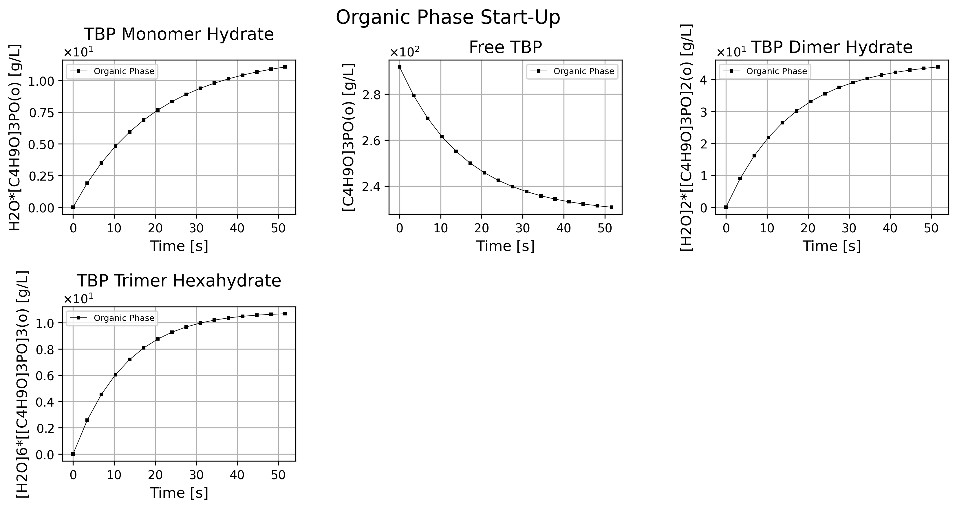
Figure 1: Organic phase species history dashboard at start-up.

if cortix_ai:
    issues = '+ Title your reponse as: Overview of the Organic Phase Data at Start-Up.'
    cortix_ai.explain(phase=stg.organic_phase, issues=issues, markdown_header_level='<h4>', markdown_display=markdown_display, save_supporting_info=db_save)

Cortix AI assistant: working on explanation...

Overview of the Organic Phase Data at Start-Up.

Summary

• The dataset spans 0 to 51.604 s with uniform time steps (~3.44027 s).

• Free ligand [C₄H₉O]₃PO(o) decreases monotonically from 291.75 to 230.811 g/L (Δ = −60.939 g/L, ≈ −20.9%).

• Three complexed species form monotonically:

  • H₂O·[C₄H₉O]₃PO(o) rises 0 -> 11.0675 g/L.

  • [H₂O]₂·[[C₄H₉O]₃PO]₂(o) rises 0 -> 43.9565 g/L (the largest complex).

  • [H₂O]₆·[[C₄H₉O]₃PO]₃(o) rises 0 -> 10.6738 g/L.

• Sum of all organic-species concentrations increases slightly from 291.75 to 296.5088 g/L (Δ ≈ +4.7588 g/L, ≈ +1.63%).

Column-by-column analysis

• Index / duplicate time column:

  • The leftmost column duplicates the “time [s]” column; both show identical values.

• time [s]:

  • Regular increments of ~3.44027 s; highest value 51.604 s.

• concentration of H₂O·[C₄H₉O]₃PO(o) [g/L]:

  • Increases from 0 to 11.0675 g/L; average rate ≈ 0.2145 g·L⁻¹·s⁻¹ over the full interval.

  • Growth rate is higher initially (≈0.552 g·L⁻¹·s⁻¹ for 0→3.44 s) and slows toward the end (~0.053 g·L⁻¹·s⁻¹ for last step).

• concentration of [C₄H₉O]₃PO(o) [g/L]:

  • Decreases steadily from 291.75 to 230.811 g/L (Δ = −60.939 g/L; ≈ −20.9%).

  • Decline is smooth and monotonic, with the largest absolute changes early on and smaller changes later.

• concentration of [H₂O]₂·[[C₄H₉O]₃PO]₂(o) [g/L]:

  • Rises to 43.9565 g/L, the largest complex concentration at final time.

  • Average growth rate ≈ 0.852 g·L⁻¹·s⁻¹; strong initial formation and pronounced deceleration by the end.

• concentration of [H₂O]₆·[[C₄H₉O]₃PO]₃(o) [g/L]:

  • Rises to 10.6738 g/L; average growth rate ≈ 0.2068 g·L⁻¹·s⁻¹.

  • Like the others, formation rate slows with time.

Comparisons and ratios

• Final partitioning (at 51.604 s):

  • Free [C₄H₉O]₃PO(o): 230.811 g/L (≈77.9% of initial single-species pool if compared to initial 291.75 alone).

  • Total complexes sum ≈ 65.6978 g/L; distribution among complexes:

    • [H₂O]₂·[[C₄H₉O]₃PO]₂(o): 43.9565 g/L (~66.9% of total complexes).

    • H₂O·[C₄H₉O]₃PO(o): 11.0675 g/L (~16.8%).

    • [H₂O]₆·[[C₄H₉O]₃PO]₃(o): 10.6738 g/L (~16.3%).

• Dominant complex: the dimer-type species [H₂O]₂·[[C₄H₉O]₃PO]₂(o) clearly dominates complex formation both in absolute concentration and fraction.

Trend implications (data-only observations)

• Kinetics implied by the data: rapid complex formation at early times followed by deceleration, consistent with approach toward a slower, near‑steady state by ~50 s.

• Mass/concise accounting: total organic concentration increases slightly (+1.63%), indicating either measurement resolution, water incorporation effects in the reported organic concentrations, or formation of species that raise measured organic-phase mass. The table itself shows monotonic and smooth evolution without oscillations or reversals.

• Overall, the table documents a conversion of free [C₄H₉O]₃PO(o) into three hydrated complexes with the two‑water complex being the predominant product and with formation rates that decrease over time, approaching a near steady composition by 50–52 s.

AI Parameters:
+ LLM model (OpenAI) = gpt-5-mini
+ LLM cleverness     = 1.0
+ Total # of tokens  = 5748

'''Compute molar concentration of TBP species'''
import numpy as np

tbp_mass_cc_org_history = stg.organic_phase.get_column(tbp_org_name)
tbp_molar_cc_org_history = np.array(tbp_mass_cc_org_history)/tbp_org.molar_mass

tbp_monomer_mass_cc_org_history = stg.organic_phase.get_column(tbp_monomer_org_name)
tbp_monomer_molar_cc_org_history = np.array(tbp_monomer_mass_cc_org_history)/tbp_monomer_org.molar_mass

tbp_dimer_mass_cc_org_history = stg.organic_phase.get_column(tbp_dimer_org_name)
tbp_dimer_molar_cc_org_history = np.array(tbp_dimer_mass_cc_org_history)/tbp_dimer_org.molar_mass

tbp_trimer_hexahydrate_mass_cc_org_history = stg.organic_phase.get_column(tbp_trimer_hexahydrate_org_name)
tbp_trimer_hexahydrate_molar_cc_org_history = np.array(tbp_trimer_hexahydrate_mass_cc_org_history)/tbp_trimer_hexahydrate_org.molar_mass

time_stamps = np.array(stg.organic_phase.time_stamps)

tbl_count += 1
print(f'Table {tbl_count}: Molarity history of TBP in the organic phase at start-up.')
print('Time [min] | Free TBP [M] | TBP Monomer [M] | TBP Dimer [M] | TBP Trimer Hexahydrate [M] | balance |')
np.set_printoptions(precision=3, suppress=True, linewidth=100)
for t,a,b,c,d in zip(time_stamps[::5]/unit.min, 
                     tbp_molar_cc_org_history[::5]/unit.molar, 
                     tbp_monomer_molar_cc_org_history[::5]/unit.molar, 
                     tbp_dimer_molar_cc_org_history[::5]/unit.molar, 
                     tbp_trimer_hexahydrate_molar_cc_org_history[::5]/unit.molar):
    balance = a+b+2*c+3*d - tbp_mass_cc_org/tbp_org.molar_mass/unit.molar
    print('  %1.2e      %1.3f         %1.3e         %1.3e             %1.3e           %+1.2e'%(t, a, b, c, d, balance))

Table 1: Molarity history of TBP in the organic phase at start-up.
Time [min] | Free TBP [M] | TBP Monomer [M] | TBP Dimer [M] | TBP Trimer Hexahydrate [M] | balance |
  0.00e+00      1.096         0.000e+00         0.000e+00             0.000e+00           +0.00e+00
  2.87e-01      0.939         2.419e-02         5.303e-02             8.904e-03           +1.11e-15
  5.73e-01      0.885         3.443e-02         7.103e-02             1.124e-02           +4.44e-16
  8.60e-01      0.867         3.892e-02         7.730e-02             1.177e-02           +8.88e-16

'''Volume fraction of TBP at start-up'''
tbl_count += 1
print(f'Table {tbl_count}: Volume fractions of free and total TBP in the organic phase at start-up.')
print('Time [min] | Free TBP vol frac [%] | Total TBP vol frac [%] |')
np.set_printoptions(precision=3, suppress=True, linewidth=100)
total_tbp_molar_cc_org_history = tbp_molar_cc_org_history + tbp_monomer_molar_cc_org_history + \
                                 2*tbp_dimer_molar_cc_org_history + 3*tbp_trimer_hexahydrate_molar_cc_org_history
total_tbp_mass_cc_org_history = total_tbp_molar_cc_org_history * tbp_org.molar_mass
for t,a,b in zip(time_stamps[::5]/unit.min, 
               np.array(tbp_mass_cc_org_history[::5])/rho_tbp*100, total_tbp_mass_cc_org_history[::5]/rho_tbp*100):
    print('  %1.2e         %1.3f                  %1.3f'%(t, a, b))

Table 2: Volume fractions of free and total TBP in the organic phase at start-up.
Time [min] | Free TBP vol frac [%] | Total TBP vol frac [%] |
  0.00e+00         30.000                  30.000
  2.87e-01         25.701                  30.000
  5.73e-01         24.244                  30.000
  8.60e-01         23.734                  30.000

'''Total water extracted'''
water_molar_cc_org_history = tbp_monomer_molar_cc_org_history \
                           + 2*tbp_dimer_molar_cc_org_history \
                           + 6*tbp_trimer_hexahydrate_molar_cc_org_history

water_mass_cc_org_history = water_molar_cc_org_history * h2o_aqu.molar_mass

tbl_count += 1
print(f'Table {tbl_count}: Mass concentration and molarity history of water in the organic phase at start-up.')
print('Time [s] |   [M]   |  [g/L]  |')
np.set_printoptions(precision=3, suppress=True, linewidth=100)
for a,b,c in zip(stg.organic_phase.time_stamps[::5], water_molar_cc_org_history[::5]/unit.molar, water_mass_cc_org_history[::5]):
    print('%1.2e  %1.3e %1.3e'%(a, b, c))

Table 3: Mass concentration and molarity history of water in the organic phase at start-up.
Time [s] |   [M]   |  [g/L]  |
0.00e+00  0.000e+00 0.000e+00
1.72e+01  1.837e-01 3.309e+00
3.44e+01  2.439e-01 4.394e+00
5.16e+01  2.641e-01 4.758e+00

'''Organic phase mass density'''
import matplotlib.pyplot as plt

quant = stg.mass_density_history('organic')

quant.plot(title='Organic Phase Mass Density @ %2.1f C Start-Up'%unit.convert_temperature(stg_temperature,
           'K','C'), x_scaling=1/stg.flow_residence_time_avg, x_label=r'Time [$\bar{\tau}$]', y_label=quant.latex_name+r'$-\rho_\text{diluent}$'
           ' ['+quant.unit+']', show=True, figsize=[10,3], error_data=False)

fig_count += 1
print(f'Figure {fig_count}: Organic phase mass density history at start-up.')

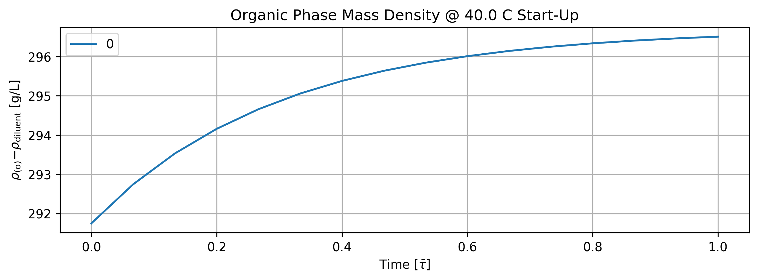
Figure 2: Organic phase mass density history at start-up.

tbl_count += 1
print(f'Table {tbl_count}: Organic phase mass density history at start-up.')
print('Time [s]  Organic Phase Mass Density [g/L]')
print(quant.value[::5].apply(lambda x: round(x,2)))

Table 4: Organic phase mass density history at start-up.
Time [s]  Organic Phase Mass Density [g/L]
0.000000     291.75
17.201342    295.06
34.402683    296.14
51.604025    296.51
Name: Organic Phase Mass Density [g/L]; Time History in [s], dtype: float64

1.5.2. Aqueous Phase Results

'''Plot aqueous phase'''
# TODO: time axis normalized by phase flow residence time.
stg.aqueous_phase.plot(title='Aqueous Phase Start-Up', legend='Aqueous Phase', nrows=2,ncols=3, show=True, figsize=[12,6])

fig_count += 1
print(f'Figure {fig_count}: Aqueous phase species history dashboard at start-up.')

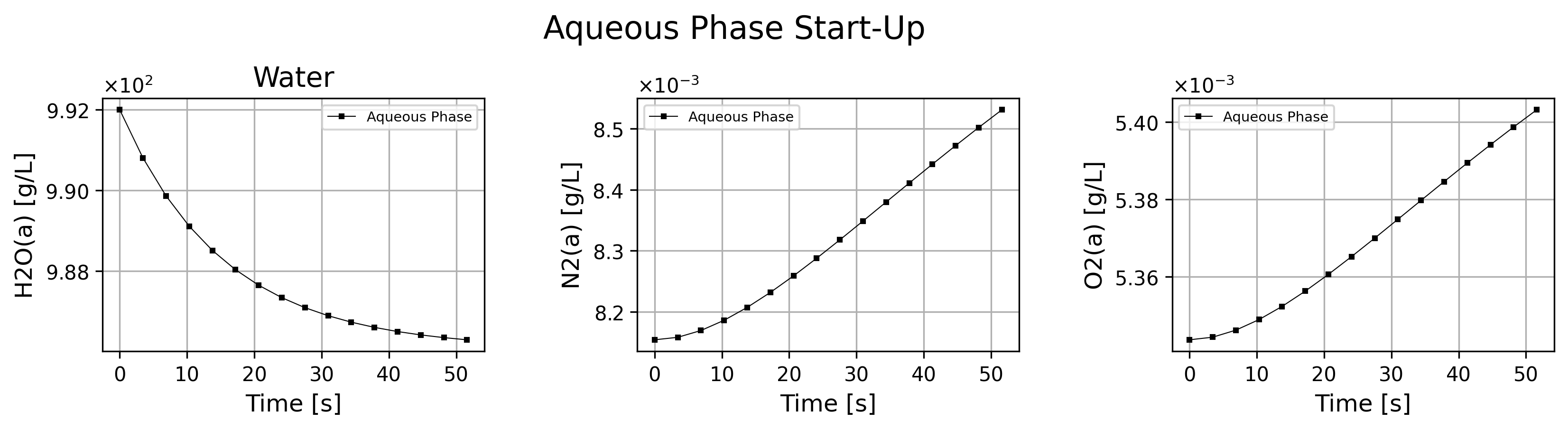
Figure 3: Aqueous phase species history dashboard at start-up.

if cortix_ai:
    issues = '+ Title your reponse as: Overview of the Aqueous Phase Data at Start-Up.'
    cortix_ai.explain(phase=stg.aqueous_phase, issues=issues, markdown_header_level='<h4>', markdown_display=markdown_display, save_supporting_info=db_save)

Cortix AI assistant: working on explanation...

Overview of the Aqueous Phase Data at Start-Up.

Summary

• The dataset spans 0 to 51.604 s and records concentrations of H₂O(a), N₂(a), and O₂(a).

• H₂O(a) decreases steadily; N₂(a) and O₂(a) increase steadily. Changes are small for dissolved gases compared with H₂O(a).

Key numeric observations

• H₂O(a): initial 992.000 g/L → final 986.288 g/L; absolute change −5.712 g/L over 51.604 s; mean rate ≈ −0.1107 g·L⁻¹·s⁻¹; relative change ≈ −0.576%.

• N₂(a): initial 0.00815443 g/L → final 0.00853078 g/L; absolute change +0.00037635 g/L; mean rate ≈ +7.29×10⁻⁶ g·L⁻¹·s⁻¹; relative change ≈ +4.62%.

• O₂(a): initial 0.00534370 g/L → final 0.00540316 g/L; absolute change +0.00005946 g/L; mean rate ≈ +1.15×10⁻⁶ g·L⁻¹·s⁻¹; relative change ≈ +1.11%.

Trends and monotonicity

• All three variables are monotonic across the recorded times: H₂O(a) strictly decreases at every sample; N₂(a) and O₂(a) strictly increase at every sample.

• Changes appear approximately linear on the sampling interval (steady per-sample increments).

Comparative remarks

• Magnitude: H₂O(a) (~10³ g/L) dominates the mass; dissolved gases are orders of magnitude smaller (~10⁻³–10⁻² g/L).

• Rate comparison: the magnitude of H₂O(a) loss (~0.11 g·L⁻¹·s⁻¹) far exceeds the combined increase rates of N₂(a)+O₂(a) (~8.44×10⁻⁶ g·L⁻¹·s⁻¹), so the gas increases do not account for the H₂O(a) decrease in a direct 1:1 mass sense over this interval.

• All columns are internally consistent with steady, short-term start-up behavior: water concentration falls modestly while dissolved-gas concentrations rise slightly.

AI Parameters:
+ LLM model (OpenAI) = gpt-5-mini
+ LLM cleverness     = 1.0
+ Total # of tokens  = 4841

'''Aqueous phase mass density'''
import matplotlib.pyplot as plt

quant = stg.mass_density_history('aqueous')

quant.plot(title='Aqueous Phase Mass Density @ %2.1f C Start-Up'%unit.convert_temperature(stg_temperature,
           'K','C'), x_scaling=1/stg.flow_residence_time_avg, x_label=r'Time [$\bar{\tau}$]', y_label=quant.latex_name+
           ' ['+quant.unit+']', show=True, figsize=[10,3], error_data=False)

fig_count += 1
print(f'Figure {fig_count}: Aqueous phase mass density history at start-up.')

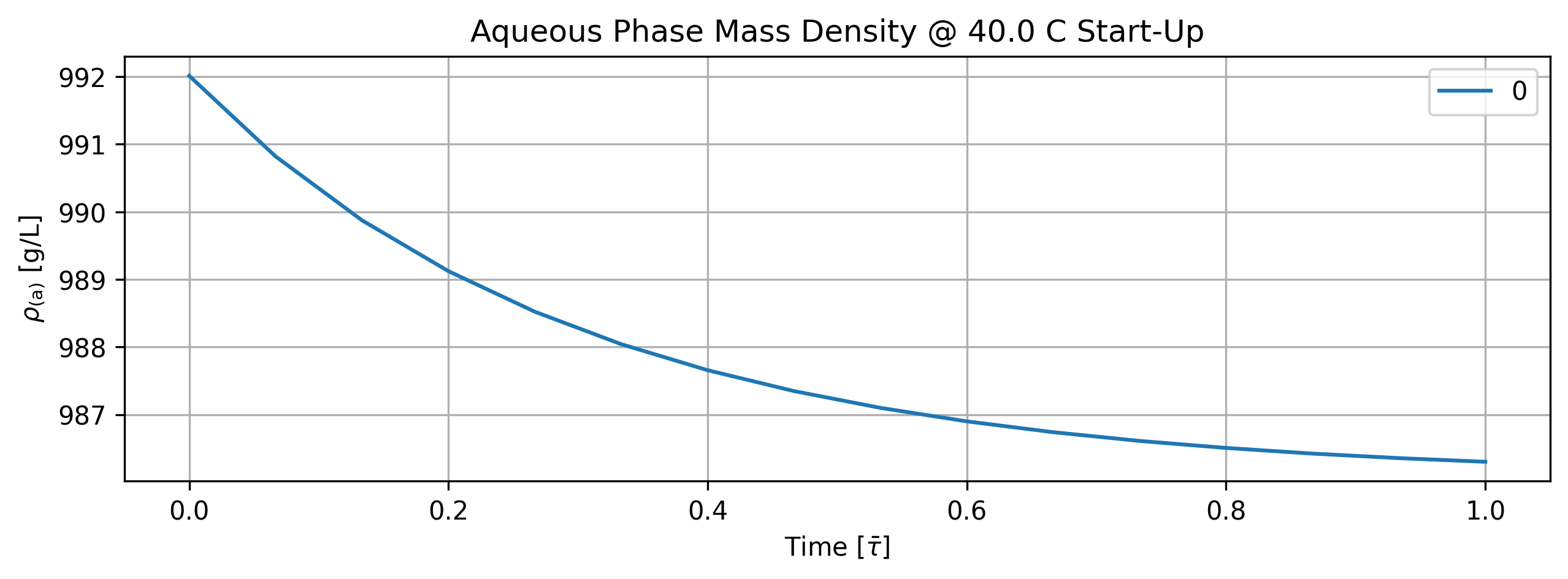
Figure 4: Aqueous phase mass density history at start-up.

tbl_count += 1
print(f'Table {tbl_count}: Aqueous phase mass density history at start-up.')
print('Time [s]  Aqueous Phase Mass Density [g/L]')
print(quant.value[::5].apply(lambda x: round(x,2)))

Table 5: Aqueous phase mass density history at start-up.
Time [s]  Aqueous Phase Mass Density [g/L]
0.000000     992.01
17.201342    988.04
34.402683    986.74
51.604025    986.30
Name: Aqueous Phase Mass Density [g/L]; Time History in [s], dtype: float64

1.5.3. Vapor Phase Results

'''Plot vapor phase'''
# TODO: time axis normalized by phase flow residence time.
stg.vapor_phase.plot(title='Vapor Phase Start-Up', legend='Vapor Phase', nrows=2,ncols=3, show=True, figsize=[12,6])

fig_count += 1
print(f'Figure {fig_count}: Vapor phase species history dashboard at start-up.')

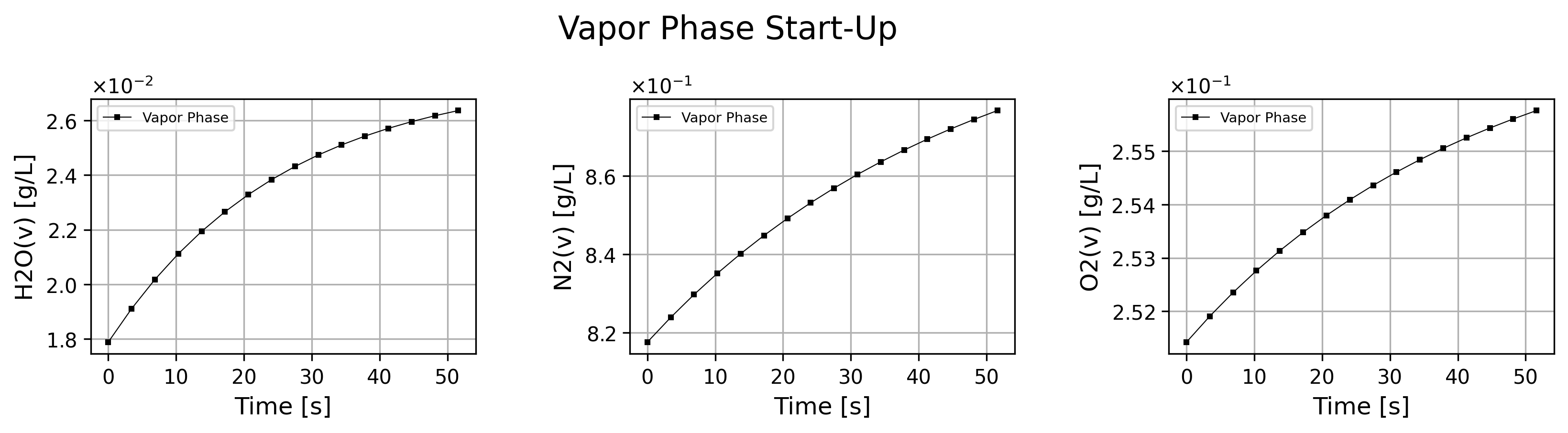
Figure 5: Vapor phase species history dashboard at start-up.

if cortix_ai:
    issues = '+ Title your reponse as: Overview of the Vapor Phase Data at Start-Up.'
    cortix_ai.explain(phase=stg.vapor_phase, issues=issues, markdown_header_level='<h4>', markdown_display=markdown_display, save_supporting_info=db_save)

Cortix AI assistant: working on explanation...

Overview of the Vapor Phase Data at Start-Up

Summary

• The table contains 16 uniformly sampled time points from 0 s to 51.604 s (Δt ≈ 3.44027 s).

• Three vapor species tracked: H₂O(v), N₂(v), O₂(v); all concentrations given in g/L and increase monotonically over the interval.

Quantitative trends (absolute and per-second rates)

• H₂O(v): rises from 0.0178756 g/L to 0.026368 g/L; absolute increase = 0.0084924 g/L; mean rate ≈ 1.6456×10⁻⁴ g·L⁻¹·s⁻¹ (≈5.662×10⁻⁴ g/L per sampling interval).

• N₂(v): rises from 0.817538 g/L to 0.876683 g/L; absolute increase = 0.059145 g/L; mean rate ≈ 1.1461×10⁻³ g·L⁻¹·s⁻¹ (≈3.943×10⁻³ g/L per sampling interval).

• O₂(v): rises from 0.25142 g/L to 0.255762 g/L; absolute increase = 0.004342 g/L; mean rate ≈ 8.414×10⁻⁵ g·L⁻¹·s⁻¹ (≈2.895×10⁻⁴ g/L per sampling interval).

Comparative analysis (relative changes and ranks)

• Relative (%) changes over the 51.604 s:

  • H₂O(v): +47.5% (largest relative increase).

  • N₂(v): +7.23%.

  • O₂(v): +1.73% (smallest relative change).

• Absolute magnitude and concentration rank (at all times): N₂(v) ≫ O₂(v) > H₂O(v); N₂(v) also has the largest absolute increase and highest absolute concentration throughout.

• Growth-rate rank (absolute rate): N₂(v) > H₂O(v) > O₂(v) by per-second slope; growth-rate rank (relative) places H₂O(v) first.

Notable observations and concise conclusions

• Sampling is uniform (consistent Δt), and each species shows a smooth, monotonic increase—no reversals or oscillations in the provided window.

• N₂(v) dominates both in instantaneous concentration and absolute accumulation; H₂O(v) shows the most pronounced percentage increase, indicating proportionally stronger enrichment from its low initial level.

• O₂(v) changes are minor in both absolute and relative terms, effectively near-constant compared with the other two species over this start-up interval.

AI Parameters:
+ LLM model (OpenAI) = gpt-5-mini
+ LLM cleverness     = 1.0
+ Total # of tokens  = 4964

'''Vapor phase mass density'''
import matplotlib.pyplot as plt

quant = stg.mass_density_history('vapor')

quant.plot(title='Vapor Phase Mass Density @ %2.1f C Start-Up'%unit.convert_temperature(stg_temperature,
           'K','C'), x_scaling=1/stg.flow_residence_time_avg, x_label=r'Time [$\bar{\tau}$]', y_label=quant.latex_name+
           ' ['+quant.unit+']', show=True, figsize=[10,3], error_data=False)

fig_count += 1
print(f'Figure {fig_count}: Vapor phase mass density history at start-up.')

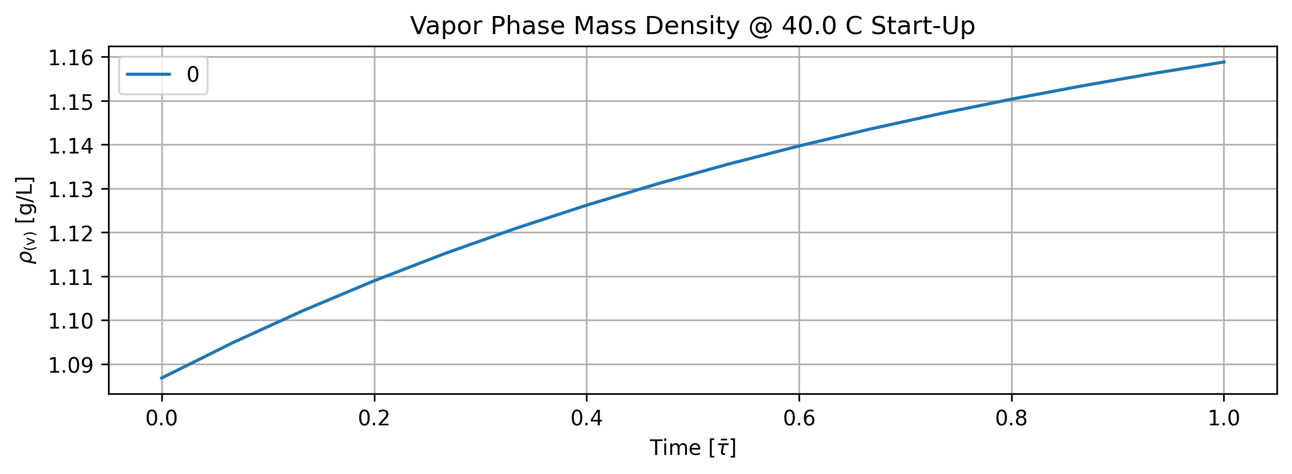
Figure 6: Vapor phase mass density history at start-up.

tbl_count += 1
print(f'Table {tbl_count}: Vapor phase mass density history at start-up.')
print('Time [s]  Vapor Phase Mass Density [g/L]')
print(quant.value[::5].apply(lambda x: round(x,2)))

Table 6: Vapor phase mass density history at start-up.
Time [s]  Vapor Phase Mass Density [g/L]
0.000000     1.09
17.201342    1.12
34.402683    1.14
51.604025    1.16
Name: Vapor Phase Mass Density [g/L]; Time History in [s], dtype: float64

1.5.3.1. Relative humidity

'''Compute relative humidity in the vapor phase'''
import matplotlib.pyplot as plt
from solvex import air_relative_humidity
from copy import deepcopy

h2o_vap_pd_series = deepcopy(stg.vapor_phase.df['H2O(v)'])
for idx, rho_h2o in enumerate(h2o_vap_pd_series):
    h2o_vap_pd_series.iloc[idx] = air_relative_humidity(stg_temperature, rho_h2o)
rh_pd_series = h2o_vap_pd_series
time_unit = stg.vapor_phase.time_unit
rh_pd_series.name = f'Relative Humidity History [{time_unit}]'
  
quant = Quantity(name=rh_pd_series.name, latex_name='RH', unit='%', info=f'Relative Humidity History (Vapor Phase) [{time_unit}]')
quant.value = h2o_vap_pd_series
quant.plot(title='Stage Rel. Humidity @ %2.1f C Start-Up'%unit.convert_temperature(stg_temperature, 'K','C'),
           x_scaling=1/stg.flow_residence_time_avg, x_label=r'Time [$\bar{\tau}$]', y_label=quant.latex_name+' ['+quant.unit+']', show=True,
           figsize=[10,3])

fig_count += 1
print(f'Figure {fig_count}: Stage relative humidity history at start-up.')

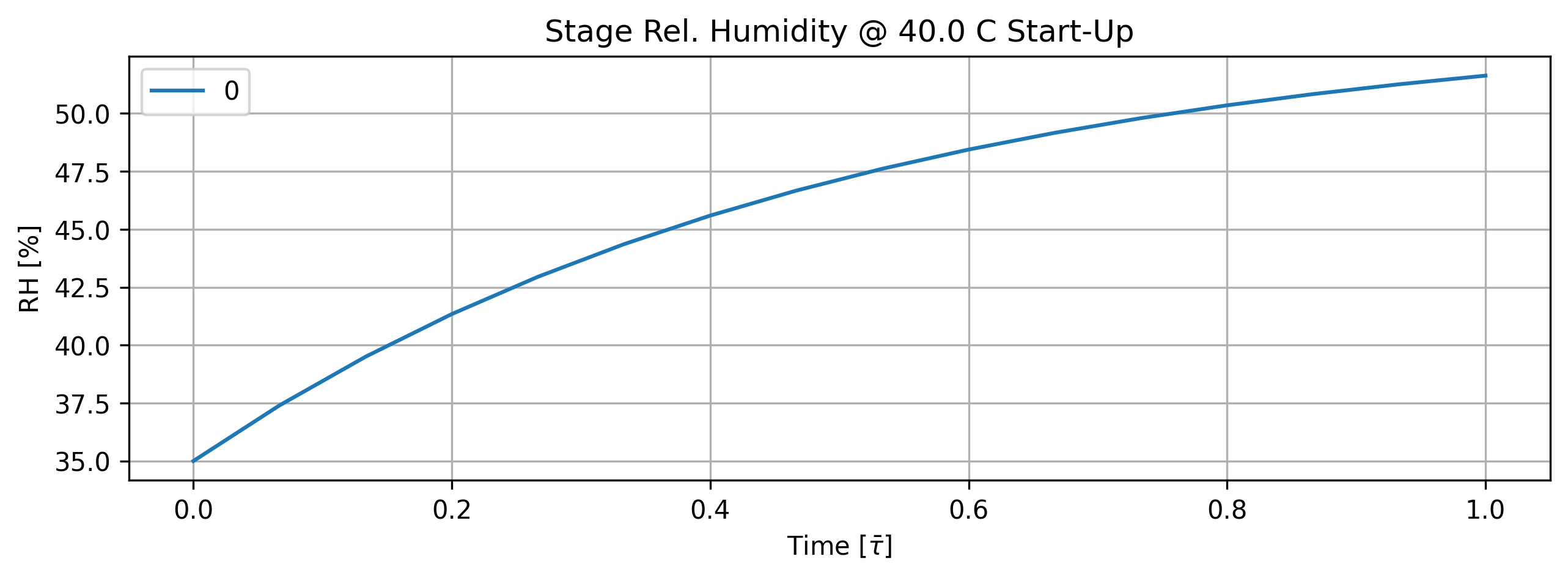
Figure 7: Stage relative humidity history at start-up.

tbl_count += 1
print(f'Table {tbl_count}: Stage relative humidity history at start-up.')
print('Time [s]  Rel. Humidity [%]')
print(quant.value[::5].apply(lambda x: round(x,2)))

Table 7: Stage relative humidity history at start-up.
Time [s]  Rel. Humidity [%]
0.000000     35.00
17.201342    44.36
34.402683    49.16
51.604025    51.63
Name: Relative Humidity History [s], dtype: float64

if cortix_ai:
    issues = '+ Title your reponse as: Overview of the Relative Humidity Data at Start-Up.'
    cortix_ai.explain(quant=quant, issues=issues, markdown_header_level='<h5>', markdown_display=markdown_display, save_supporting_info=db_save)

Cortix AI assistant: working on explanation...

Overview of the Relative Humidity Data at Start-Up.

Data summary

Measured quantity: Relative Humidity (vapor phase) in percent (%) sampled at eight times during start-up.

• Key columns and coverage

  • Index: row identifier 0…7.

  • time [s]: uniformly sampled from 0.0000 s to 48.1638 s (step ≈ 6.88054 s).

  • Relative Humidity [%]: values from 35.0000% to 51.2567%.

Descriptive statistics

• Basic statistics

  • Count: 8 samples.

  • Minimum: 35.0000% at t = 0.0000 s.

  • Maximum: 51.2567% at t = 48.1638 s.

  • Mean (average): 45.1773%.

  • Median: 46.6009% (average of the 4th and 5th ordered values).

  • Standard deviation: ≈ 5.32% (population) or ≈ 5.69% (sample, N−1).

Temporal behaviour and rates

• Overall change and average rate

  • Total increase: 16.2567 percentage points over 48.1638 s.

  • Average rate (overall): ≈ 0.338 %/s.

• Per-interval changes (time intervals ≈ 6.88054 s)

  • t = 0.0000 -> 6.8805 s: ΔRH = +4.5013% -> ≈ 0.655 %/s

  • t = 6.8805 -> 13.7611 s: ΔRH = +3.4477% -> ≈ 0.501 %/s

  • t = 13.7611 -> 20.6416 s: ΔRH = +2.6406% -> ≈ 0.384 %/s

  • t = 20.6416 -> 27.5221 s: ΔRH = +2.0226% -> ≈ 0.294 %/s

  • t = 27.5221 -> 34.4027 s: ΔRH = +1.5491% -> ≈ 0.225 %/s

  • t = 34.4027 -> 41.2832 s: ΔRH = +1.1866% -> ≈ 0.173 %/s

  • t = 41.2832 -> 48.1638 s: ΔRH = +0.9088% -> ≈ 0.132 %/s

Observations

• The relative humidity increases monotonically during the recorded start-up period.

• The rate of increase declines with time (largest rise initially, then progressively smaller increments), indicating an approach toward a quasi‑steady RH near the recorded maximum (~51.3%) in this time window.

• Time sampling is effectively uniform (Δt ≈ 6.88054 s), so the observed deceleration in ΔRH per interval reflects true slowdown of RH change rather than variable sampling.

AI Parameters:
+ LLM model (OpenAI) = gpt-5-mini
+ LLM cleverness     = 1.0
+ Total # of tokens  = 5087

1.5.4. Overall Stage Efficiency

Stage efficiency measures how close to chemical equilibrium the system is as a whole. This is a direct result of the reaction relaxation time which is dependent on the mass transfer coefficients of the system. Much more needs to be investigated in this project with various degrees of theory but these results represent the beginning of a solid development.

'''Stage overall efficiency'''

quant = stg.efficiency_history(mean=True)
quant.plot(title='Stage Efficiency @ %2.1f C Start-Up'%unit.convert_temperature(stg_temperature,
           'K','C'), x_scaling=1/stg.flow_residence_time_avg, x_label=r'Time [$\bar{\tau}$]', y_label=quant.latex_name+
           ' ['+quant.unit+']', show=True, figsize=[10,3], error_data=True)

fig_count += 1
print(f'Figure {fig_count}: Stage efficiency history at start-up.')

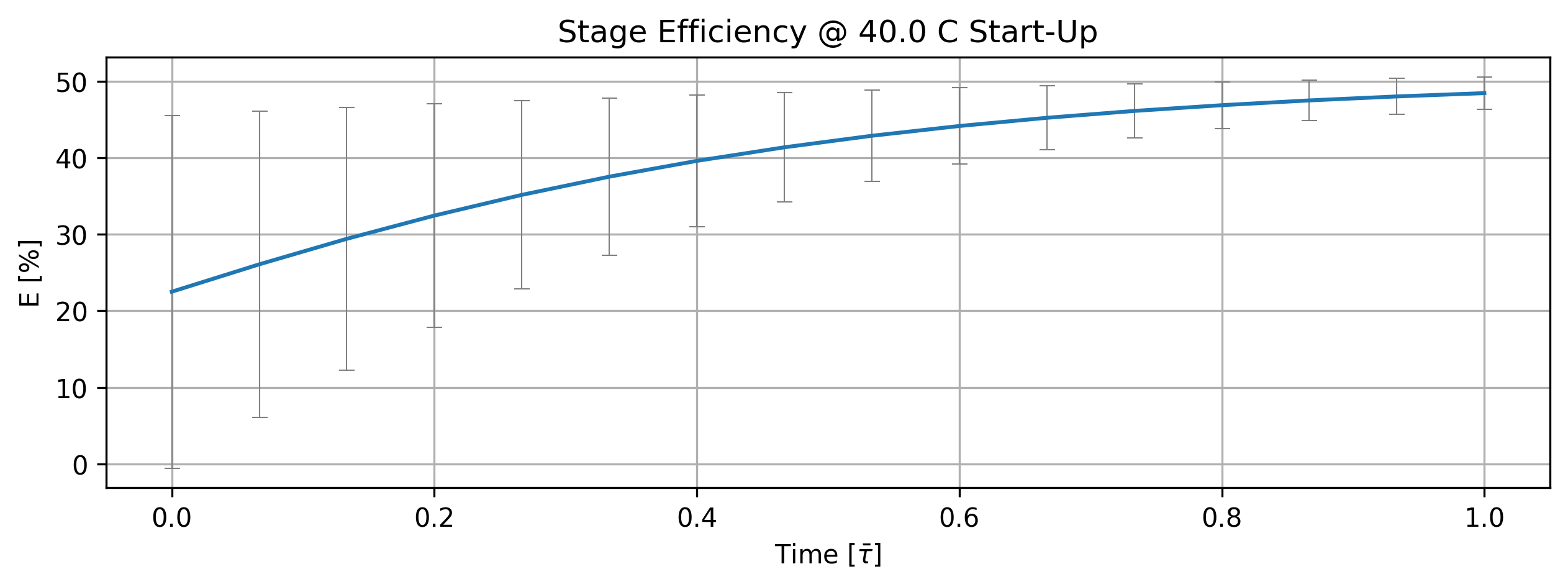
Figure 8: Stage efficiency history at start-up.

tbl_count += 1
print(f'Table {tbl_count}: Stage efficiency history at start-up.')
print('Time [s]  (Stage. Eff., +-std) [%]')
time_name = ''
import pandas as pd
df = (quant.value.apply(pd.Series).mul(1)
       .rename(index=lambda i: round(i/unit.min,2))
       .set_axis(['',''], axis=1).rename_axis(time_name)
       .round(3))
print(df.to_string(max_rows=20, min_rows=20))

Table 8: Stage efficiency history at start-up.
Time [s]  (Stage. Eff., +-std) [%]
                    
                    
0.00  22.500  23.049
0.06  26.079  20.002
0.11  29.411  17.158
0.17  32.443  14.575
0.23  35.149  12.284
0.29  37.528  10.291
0.34  39.592   8.587
0.40  41.363   7.153
0.46  42.871   5.962
0.52  44.146   4.984
0.57  45.218   4.192
0.63  46.116   3.557
0.69  46.866   3.055
0.75  47.491   2.663
0.80  48.010   2.360
0.86  48.441   2.131

if cortix_ai:
    issues = '+ Title your reponse as: Overview of the Stage Efficiency Data at Start-Up.'
    cortix_ai.explain(quant=quant, issues=issues, markdown_header_level='<h4>', markdown_display=markdown_display, print_prompt=False, save_supporting_info=db_save)

Cortix AI assistant: working on explanation...

Overview of the Stage Efficiency Data at Start-Up

Dataset summary

• The table reports a time history (time in s) of stage efficiency (dependent quantity in %) with two columns: column “0” = mean efficiency (%) and column “1” = associated standard deviation (± std, %).

• Time points: 0.0000, 6.88054, 13.7611, 20.6416, 27.5221, 34.4027, 41.2832, 48.1638 s (8 samples).

• Mean efficiency range: 22.5% → 48.0099% (min → max).

• Standard-deviation range: 23.0489% → 2.36039% (initial → final).

Column-wise analysis

• Time [s]

  • Evenly spaced by ~6.88054 s increments; spans 0 → 48.1638 s.

• Mean efficiency (column “0”, %)

  • Values: 22.5, 29.411, 35.1492, 39.5916, 42.8713, 45.2185, 46.8661, 48.0099.

  • Monotonic increase at every sample (no decreases observed).

  • Net change: +25.5099 percentage points over 48.1638 s → average rate ≈ 0.53 % per s.

• Standard deviation (column “1”, %)

  • Values: 23.0489, 17.1583, 12.2838, 8.58727, 5.96182, 4.19209, 3.05491, 2.36039.

  • Monotonic decrease at every sample (uncertainty falls continuously).

  • Net change: −20.68851 percentage points over 48.1638 s → average rate ≈ −0.43 % per s.

• Relative spread (std / mean, coefficient of variation)

  • t = 0 s: 102.4%

  • t = 6.88 s: 58.3%

  • t = 13.76 s: 35.0%

  • t = 20.64 s: 21.7%

  • t = 27.52 s: 13.9%

  • t = 34.40 s: 9.3%

  • t = 41.28 s: 6.5%

  • t = 48.16 s: 4.9%

  • Interpretation: relative uncertainty falls from >100% at start-up to <5% by ~48 s.

Key observations

• The mean stage efficiency increases steadily during the start-up interval, roughly doubling from 22.5% to 48.0%.

• The standard deviation decreases steadily, indicating that estimates become more precise/stable as time progresses.

• The sharpest fractional reduction in uncertainty occurs early (first two samples), with progressively smaller absolute reductions later.

• By ~20–28 s the mean is ~40–43% and relative uncertainty has dropped to ~14–22%, with further stabilization thereafter.

AI Parameters:
+ LLM model (OpenAI) = gpt-5-mini
+ LLM cleverness     = 1.0
+ Total # of tokens  = 4639

'''Individual reaction efficiency'''

quant = stg.efficiency_history()
quant.plot(title='Reaction Efficiency @ %2.1f C Start-Up'%unit.convert_temperature(stg_temperature,
           'K','C'), x_scaling=1/stg.flow_residence_time_avg, x_label=r'Time [$\bar{\tau}$]', y_label=quant.latex_name+
           ' ['+quant.unit+']', legend=stg.rxn_mech.reactions, show=True, figsize=[10,3])

fig_count += 1
print(f'Figure {fig_count}: Reaction efficiency history at start-up.')

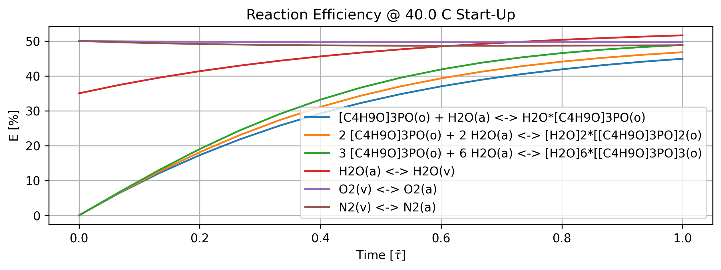
Figure 9: Reaction efficiency history at start-up.

'''Individual reaction efficiency'''

quant = stg.efficiency_history()

tbl_count += 1
print(f'Table {tbl_count}: Reaction efficiency history at start-up.')
print('Time [min]    Rxn Eff. [%]')

col_names = [f'r{i}' for i in range(len(stg.rxn_mech.reactions))]
time_name = ''
df = (quant.value.apply(pd.Series).mul(1)
       .rename(index=lambda i: round(i/unit.min,2))
       .set_axis(col_names, axis=1).rename_axis(time_name)
       .round(3))
print(df.to_string(max_rows=20, min_rows=20))

Table 9: Reaction efficiency history at start-up.
Time [min]    Rxn Eff. [%]
          r0      r1      r2      r3      r4      r5
                                                    
0.00   0.000   0.000   0.000  35.000  50.000  50.000
0.06   6.372   6.506   6.644  37.401  49.910  49.642
0.11  12.131  12.581  13.054  39.502  49.839  49.359
0.17  17.270  18.111  19.012  41.340  49.783  49.140
0.23  21.807  23.042  24.383  42.949  49.741  48.972
0.29  25.779  27.366  29.107  44.358  49.710  48.847
0.34  29.232  31.105  33.176  45.590  49.688  48.758
0.40  32.218  34.303  36.618  46.669  49.674  48.698
0.46  34.790  37.011  39.488  47.613  49.665  48.661
0.52  36.997  39.288  41.849  48.439  49.661  48.644
0.57  38.886  41.190  43.768  49.162  49.662  48.643
0.63  40.501  42.772  45.312  49.795  49.665  48.654
0.69  41.880  44.080  46.542  50.348  49.671  48.675
0.75  43.055  45.160  47.512  50.833  49.678  48.704
0.80  44.058  46.048  48.270  51.257  49.688  48.739
0.86  44.912  46.776  48.855  51.628  49.698  48.779

if cortix_ai:
    issues = '+ Title your reponse as: Overview of Individual Reaction Efficiency at Start-Up.'
    cortix_ai.explain(quant=quant, issues=issues, markdown_header_level='<h4>', markdown_display=markdown_display, print_prompt=False, save_supporting_info=db_save)

Cortix AI assistant: working on explanation...

Overview of Individual Reaction Efficiency at Start-Up.

Data shown: Rxns Efficiency [%] as a function of time (s). Time points: 0, 6.88054, 13.7611, 20.6416, 27.5221, 34.4027, 41.2832, 48.1638.

• Column → reaction mapping

  • Column 0: [C₄H₉O]₃PO(o) + H₂O(a) <-> H₂O·[C₄H₉O]₃PO(o)

  • Column 1: 2 [C₄H₉O]₃PO(o) + 2 H₂O(a) <-> [H₂O]₂·[[C₄H₉O]₃PO]₂(o)

  • Column 2: 3 [C₄H₉O]₃PO(o) + 6 H₂O(a) <-> [H₂O]₆·[[C₄H₉O]₃PO]₃(o)

  • Column 3: H₂O(a) <-> H₂O(v)

  • Column 4: O₂(v) <-> O₂(a)

  • Column 5: N₂(v) <-> N₂(a)

• Time-series summary (per reaction; values are efficiencies [%] at t = 0 → 48.1638 s)

  • Reaction 0 (column 0)

    • Values: 0 → 12.13 → 21.81 → 29.23 → 34.79 → 38.89 → 41.88 → 44.06

    • Behavior: monotonic increase from 0% to 44.06% over the interval; growth rate is initially large and slows toward the end.

  • Reaction 1 (column 1)

    • Values: 0 → 12.58 → 23.04 → 31.11 → 37.01 → 41.19 → 44.08 → 46.05

    • Behavior: monotonic increase to 46.05%; similar trend to Reaction 0 but reaches a higher efficiency by 48 s.

  • Reaction 2 (column 2)

    • Values: 0 → 13.05 → 24.38 → 33.18 → 39.49 → 43.77 → 46.54 → 48.27

    • Behavior: monotonic increase, attaining the highest efficiency among the three condensed-phase cluster formations (48.27% at final time).

  • Reaction 3 (column 3)

    • Values: 35.0003 → 39.50 → 42.95 → 45.59 → 47.61 → 49.16 → 50.35 → 51.26

    • Behavior: starts already high (35%), increases steadily and crosses the 50% mark between 34.4 s and 41.28 s, ending at 51.26%.

  • Reaction 4 (column 4)

    • Values: 50 → 49.84 → 49.74 → 49.69 → 49.67 → 49.66 → 49.67 → 49.69

    • Behavior: starts at 50% then dips slightly and stabilizes near 49.66–49.69%; essentially steady with minor fluctuations just below 50%.

  • Reaction 5 (column 5)

    • Values: 50 → 49.36 → 48.97 → 48.76 → 48.66 → 48.64 → 48.68 → 48.74

    • Behavior: begins at 50%, then declines to ~48.64% and shows a small recovery to 48.74% by the last time point; overall slightly decreasing then flattening.

• Key comparative observations

  • The three cluster-formation reactions (columns 0, 1, 2) start at 0% and increase monotonically; column 2 rises fastest to ~48.3% by 48 s, followed by column 1 (~46.0%) and column 0 (~44.1%).

  • The gas–liquid exchange for H₂O (column 3) is the only reaction that exceeds 50% by the end of the record (finishes at 51.26%), having begun at a comparatively high 35%.

  • O₂ and N₂ exchange reactions (columns 4 and 5) remain near 50% at start-up and settle just below 50% (around 49.66 and 48.74%, respectively), showing very small variation compared with the other reactions.

  • Crossing of the 50% threshold is observed only for Reaction 3 within the observed time window; Reactions 4 and 5 are effectively steady near 50% but do not sustain >50% except at t = 0.

• Final-state snapshot (t = 48.1638 s)

  • Reaction 0: 44.06%

  • Reaction 1: 46.05%

  • Reaction 2: 48.27%

  • Reaction 3: 51.26%

  • Reaction 4: 49.69%

  • Reaction 5: 48.74%

Overall, the dataset shows rapid startup growth for the condensed-phase complexation reactions and a dominant H₂O vapor–liquid exchange that surpasses 50% efficiency within the 48 s window; O₂ and N₂ exchanges are essentially stable just below 50%.

AI Parameters:
+ LLM model (OpenAI) = gpt-5-mini
+ LLM cleverness     = 1.0
+ Total # of tokens  = 5689

1.5.4.1. Total water extracted in equilibrium

From reference: 1994 Naganawa and Tachimori Anal. Sci. 10 p 607

[H2O]_o,E = 0.4265 M

h2o_e_molar = water_molar_cc_org_history[-1]/unit.molar

print('Total H2O extracted [M] = %1.4f'%h2o_e_molar)
print('Error (compared to measurement) [%%] = %1.2f'%((h2o_e_molar-0.4265)/0.4265*100))

Total H2O extracted [M] = 0.2641
Error (compared to measurement) [%] = -38.07

1.5.5. Reaction Rate Density

This quantity only makes sense per volume of the mixture.

'''Reaction rate density'''
import matplotlib.pyplot as plt

quant = stg.r_vec_history() # mole/m^3-s

quant.plot(title='Reaction Rate Density @ %2.1f C Start-Up'%unit.convert_temperature(stg_temperature,
           'K','C'), x_scaling=1/stg.flow_residence_time_avg, x_label=r'Time [$\bar{\tau}$]', y_label=quant.latex_name+
           ' ['+quant.unit+']', legend=stg.rxn_mech.reactions, show=True, figsize=[10,3], error_data=False)

fig_count += 1
print(f'Figure {fig_count}: Reaction rate density history at start-up.')

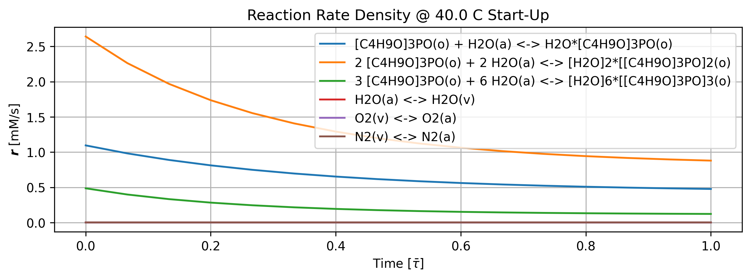
Figure 10: Reaction rate density history at start-up.

tbl_count += 1
print(f'Table {tbl_count}: Reaction rate density history at start-up.')
print('Time [min]      r [mM/s]')
import pandas as pd
col_names = [f'r{i}' for i in range(len(stg.rxn_mech.reactions))]
time_name = 't [min]'
df = (quant.value.apply(pd.Series).mul(1)
       .rename(index=lambda i: round(i/unit.min,2))
       .set_axis(col_names, axis=1).rename_axis(time_name)
       .round(4))
print(df.to_string(max_rows=20, min_rows=20))

Table 10: Reaction rate density history at start-up.
Time [min]      r [mM/s]
             r0      r1      r2      r3      r4      r5
t [min]                                                
0.00     1.0955  2.6403  0.4865  0.0019  0.0014  0.0024
0.06     0.9820  2.2626  0.3985  0.0019  0.0014  0.0025
0.11     0.8889  1.9681  0.3330  0.0018  0.0014  0.0025
0.17     0.8122  1.7365  0.2836  0.0017  0.0014  0.0025
0.23     0.7490  1.5533  0.2459  0.0017  0.0014  0.0025
0.29     0.6966  1.4076  0.2169  0.0016  0.0014  0.0026
0.34     0.6532  1.2912  0.1944  0.0016  0.0014  0.0026
0.40     0.6171  1.1980  0.1770  0.0016  0.0014  0.0026
0.46     0.5870  1.1231  0.1633  0.0016  0.0014  0.0026
0.52     0.5620  1.0627  0.1527  0.0015  0.0014  0.0026
0.57     0.5411  1.0141  0.1444  0.0015  0.0014  0.0026
0.63     0.5235  0.9748  0.1378  0.0015  0.0014  0.0026
0.69     0.5088  0.9430  0.1327  0.0015  0.0014  0.0026
0.75     0.4965  0.9173  0.1287  0.0015  0.0014  0.0027
0.80     0.4862  0.8964  0.1256  0.0014  0.0014  0.0027
0.86     0.4774  0.8795  0.1232  0.0014  0.0014  0.0027

if cortix_ai:
    issues = '+ Title your reponse as: Overview of Reaction Rates Density at Start-Up.'
    cortix_ai.explain(quant=quant, issues=issues, markdown_header_level='<h4>', markdown_display=markdown_display, print_prompt=False, save_supporting_info=db_save)

Cortix AI assistant: working on explanation...

Overview of Reaction Rates Density at Start-Up

Time history of reaction-rate densities (unit: mM/s) sampled at t = 0, 6.8805, 13.7611, 20.6416, 27.5221, 34.4027, 41.2832, 48.1638 s. Columns 0–5 map to the ordered reactions (converted “*” -> “·” and digits subscripted) shown below; values are the table entries for each reaction at each time.

• Quick summary

  • Columns 0–2 (the three [C₄H₉O]₃PO-based association reactions) have the largest rates (≈10⁻¹–10⁰ mM/s) and show clear monotonic decay toward smaller values over the 48 s window.

  • Columns 3–5 (gas–adsorbate exchanges H₂O, O₂, N₂) are ≈10⁻³ mM/s (three orders of magnitude smaller); column 3 decreases moderately, while columns 4 and 5 are nearly constant to slightly increasing.

  • Time spacing is nearly uniform (~6.8805 s between samples); the largest fractional changes occur earlier and decay slows toward the end of the record.

• Per-reaction details (column index -> reaction; initial value at t=0 -> final at t≈48.16 s; % change; trend / remarks)

  • Column 0 -> [C₄H₉O]₃PO(o) + H₂O(a) <-> H₂O·[C₄H₉O]₃PO(o): 1.09551 -> 0.48616 (−55.6%); monotonic decrease, large absolute rate and substantial decay toward a lower steady value.

  • Column 1 -> 2 [C₄H₉O]₃PO(o) + 2 H₂O(a) <-> [H₂O]₂·[[C₄H₉O]₃PO]₂(o): 2.64031 -> 0.896419 (−66.0%); largest initial rate, strong decay, similar kinetics shape to column 0 but larger magnitude.

  • Column 2 -> 3 [C₄H₉O]₃PO(o) + 6 H₂O(a) <-> [H₂O]₆·[[C₄H₉O]₃PO]₃(o): 0.486462 -> 0.125621 (−74.2%); moderate initial rate, fastest fractional decay of the three association reactions.

  • Column 3 -> H₂O(a) <-> H₂O(v): 0.00192565 -> 0.00144403 (−25.0%); small magnitude, modest decrease indicating a reducing net transfer rate (toward weaker net exchange) over the interval.

  • Column 4 -> O₂(v) <-> O₂(a): 0.00139164 -> 0.00142364 (+2.3%); essentially steady with a slight increase (near measurement/variation scale compared with columns 0–2).

  • Column 5 -> N₂(v) <-> N₂(a): 0.00242574 -> 0.00265994 (+9.6%); small absolute rate, slight upward trend across the sampling window.

• Magnitude grouping and implication

  • High-magnitude group: columns 0–2 (association/aggregation reactions involving [C₄H₉O]₃PO) dominate the reaction-rate density budget; their decrease implies the start-up transient is driving these processes toward lower net rates within ~50 s.

  • Low-magnitude group: columns 3–5 (phase/adsorption exchanges for H₂O, O₂, N₂) are minor contributors to total mM/s but show different behaviors: H₂O exchange weakens, while O₂ and N₂ exchanges are near-constant or slightly increase.

• Temporal behavior (qualitative)

  • The three association reactions show a fast initial drop followed by slower decline (consistent with a relaxation toward a quasi-steady state over tens of seconds).

  • Gas–adsorbate exchanges are relatively stable; small variability may reflect small net driving-force changes or coupling to the larger association kinetics.

• Numeric notes

  • Sampling times: [0.00000, 6.88054, 13.76110, 20.64160, 27.52210, 34.40270, 41.28320, 48.16380] s.

  • Absolute scales span ≈0.0014–2.64 mM/s; the largest single rate is 2.64031 mM/s (col. 1 at t=0).

• Bottom-line

  • Start-up dynamics are dominated by rapid decay of the [C₄H₉O]₃PO-related association reactions (cols 0–2) over the first ≈50 s, while the gas–adsorbate exchange rates (cols 3–5) remain small and comparatively steady.

AI Parameters:
+ LLM model (OpenAI) = gpt-5-mini
+ LLM cleverness     = 1.0
+ Total # of tokens  = 5633

1.5.6. Species Generation Rate Density

This quantity is on the basis of mixing volume so all species generation values can be compared.

'''Species generation rate density'''
import matplotlib.pyplot as plt

quant = stg.g_vec_history() # mole/m^3-s

quant.plot(title='Species Generation Rate Density @ %2.1f C Start-Up'%unit.convert_temperature(stg_temperature,
           'K','C'), x_scaling=1/stg.flow_residence_time_avg, x_label=r'Time [$\bar{\tau}$]', y_label=quant.latex_name+
           ' ['+quant.unit+']', legend=stg.rxn_mech.species_names, show=True, figsize=[10,3], error_data=False)

fig_count += 1
print(f'Figure {fig_count}: Species generation rate density history at start-up.')

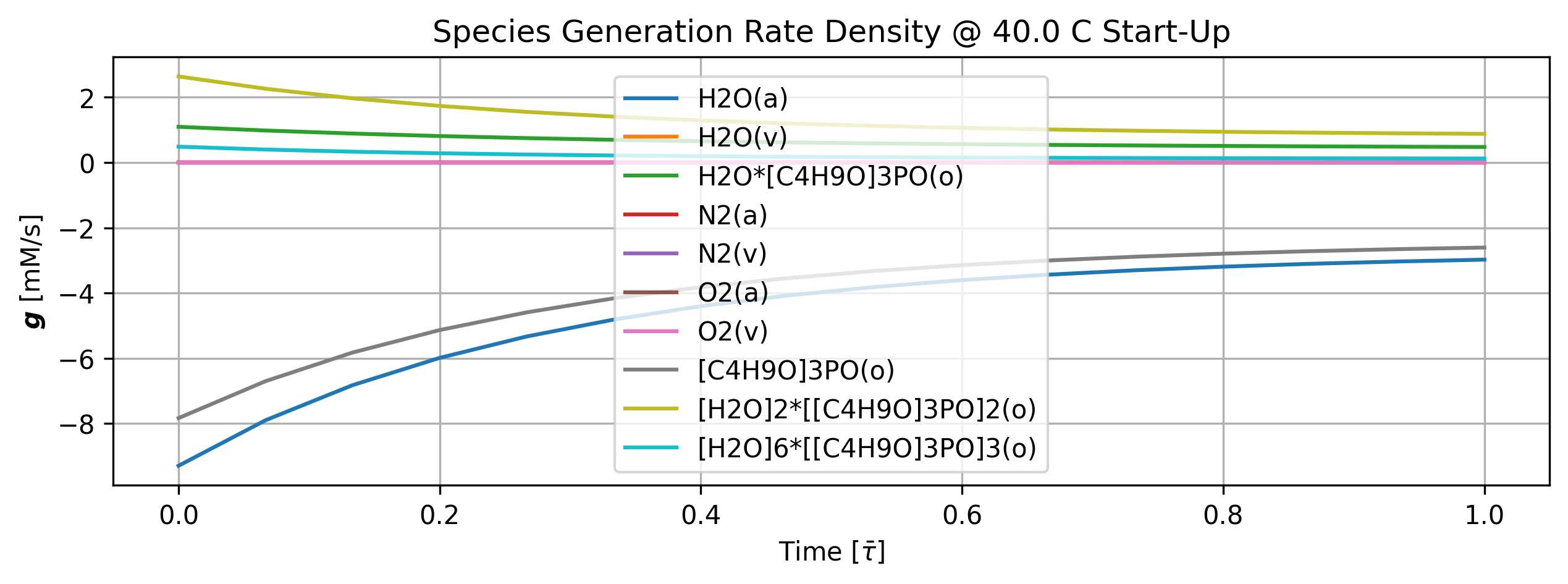
Figure 11: Species generation rate density history at start-up.

tbl_count += 1
print(f'Table {tbl_count}: Species generation rate density history at start-up.')
print('Time [min]        g [mM/s]')
import pandas as pd
col_names = [f'a{i}' for i in range(len(stg.rxn_mech.species_names))]
time_name = 't [min]'
df = (quant.value.apply(pd.Series).mul(1)
       .rename(index=lambda i: round(i/unit.min,2))
       .set_axis(col_names, axis=1).rename_axis(time_name)
       .round(4))
print(df.to_string(max_rows=20, min_rows=20))

Table 11: Species generation rate density history at start-up.
Time [min]        g [mM/s]
             a0      a1      a2      a3      a4      a5      a6      a7      a8      a9
t [min]                                                                                
0.00    -9.2968  0.0019  1.0955  0.0024 -0.0024  0.0014 -0.0014 -7.8355  2.6403  0.4865
0.06    -7.9002  0.0019  0.9820  0.0025 -0.0025  0.0014 -0.0014 -6.7028  2.2626  0.3985
0.11    -6.8249  0.0018  0.8889  0.0025 -0.0025  0.0014 -0.0014 -5.8240  1.9681  0.3330
0.17    -5.9884  0.0017  0.8122  0.0025 -0.0025  0.0014 -0.0014 -5.1359  1.7365  0.2836
0.23    -5.3323  0.0017  0.7490  0.0025 -0.0025  0.0014 -0.0014 -4.5931  1.5533  0.2459
0.29    -4.8145  0.0016  0.6966  0.0026 -0.0026  0.0014 -0.0014 -4.1623  1.4076  0.2169
0.34    -4.4036  0.0016  0.6532  0.0026 -0.0026  0.0014 -0.0014 -3.8188  1.2912  0.1944
0.40    -4.0763  0.0016  0.6171  0.0026 -0.0026  0.0014 -0.0014 -3.5439  1.1980  0.1770
0.46    -3.8148  0.0016  0.5870  0.0026 -0.0026  0.0014 -0.0014 -3.3232  1.1231  0.1633
0.52    -3.6052  0.0015  0.5620  0.0026 -0.0026  0.0014 -0.0014 -3.1456  1.0627  0.1527
0.57    -3.4369  0.0015  0.5411  0.0026 -0.0026  0.0014 -0.0014 -3.0023  1.0141  0.1444
0.63    -3.3016  0.0015  0.5235  0.0026 -0.0026  0.0014 -0.0014 -2.8866  0.9748  0.1378
0.69    -3.1927  0.0015  0.5088  0.0026 -0.0026  0.0014 -0.0014 -2.7930  0.9430  0.1327
0.75    -3.1049  0.0015  0.4965  0.0027 -0.0027  0.0014 -0.0014 -2.7173  0.9173  0.1287
0.80    -3.0342  0.0014  0.4862  0.0027 -0.0027  0.0014 -0.0014 -2.6559  0.8964  0.1256
0.86    -2.9771  0.0014  0.4774  0.0027 -0.0027  0.0014 -0.0014 -2.6061  0.8795  0.1232

'''Produced species generation rate density'''
import matplotlib.pyplot as plt

ids, quant_produced = stg.g_vec_history(produced=True) # mole/m^3-s

quant_produced.plot(title='Produced Species Generation Rate Density @ %2.1f C Start-Up'%unit.convert_temperature(stg_temperature,
           'K','C'), x_scaling=1/stg.flow_residence_time_avg, x_label=r'Time [$\bar{\tau}$]', y_label=quant.latex_name+
           ' ['+quant_produced.unit+']', legend=list(np.array(stg.rxn_mech.species_names)[ids]), show=True, figsize=[10,3], error_data=False)

fig_count += 1
print(f'Figure {fig_count}: Produced species generation rate density history at start-up.')

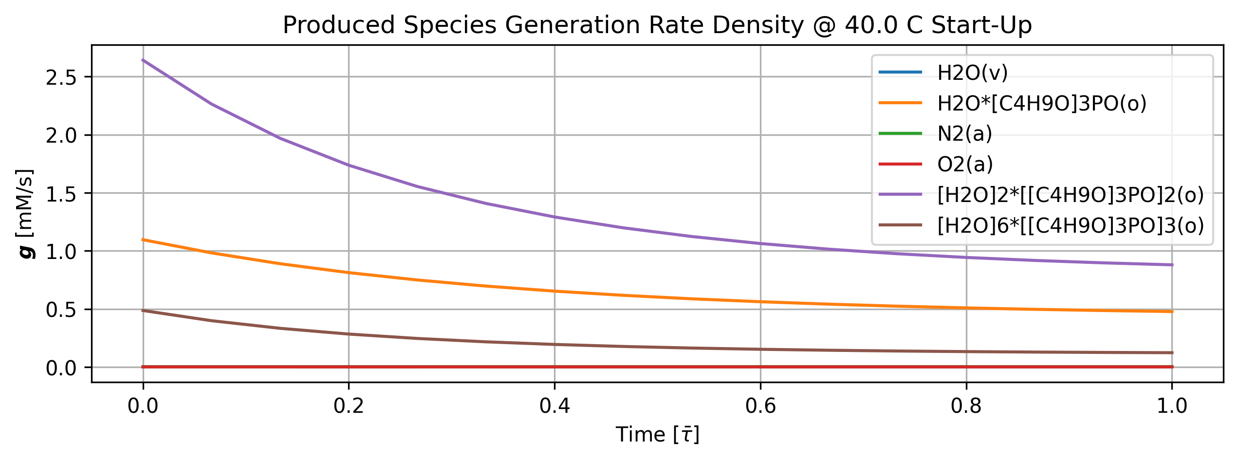
Figure 12: Produced species generation rate density history at start-up.

if cortix_ai:
    issues = '+ Title your reponse as: Overview of Species Generation Rates Density at Start-Up.'
    cortix_ai.explain(quant=quant, issues=issues, markdown_header_level='<h4>', markdown_display=markdown_display, print_prompt=False, save_supporting_info=db_save)

Cortix AI assistant: working on explanation...

Overview of Species Generation Rates Density at Start-Up

Dataset summary

• Time span: 0 s to 48.1638 s in 8 sampling instants; dependent variable: species generation-rate density in mM/s.

• Ten species (columns 0–9) in the given order: H₂O(a), H₂O(v), H₂O·[C₄H₉O]₃PO(o), N₂(a), N₂(v), O₂(a), O₂(v), [C₄H₉O]₃PO(o), [H₂O]₂·[[C₄H₉O]₃PO]₂(o), [H₂O]₆·[[C₄H₉O]₃PO]₃(o).

• Values show a start-up transient: large-magnitude condensed-phase production/consumption at t = 0 that decays toward smaller magnitudes by t ≈ 48 s; small gaseous-phase pairs show near-equal opposite rates.

Per-species time trends (initial → final; Δ = final − initial)

• H₂O(a): −9.29682 → −3.03417; Δ = +6.26265 (strong net consumption at t=0 that weakens steadily).

• H₂O(v): 0.00192565 → 0.00144403; Δ = −0.00048162 (small positive production, slowly decreasing).

• H₂O·[C₄H₉O]₃PO(o): 1.09551 → 0.48616; Δ = −0.60935 (positive production that decays substantially).

• N₂(a): 0.00242574 → 0.00265994; Δ = +0.00023420 (small positive production, slight increase).

• N₂(v): −0.00242574 → −0.00265994; Δ = −0.00023420 (equal-and-opposite to N₂(a) throughout).

• O₂(a): 0.00139164 → 0.00142364; Δ = +0.00003200 (very small positive production, nearly constant).

• O₂(v): −0.00139164 → −0.00142364; Δ = −0.00003200 (equal-and-opposite to O₂(a) throughout).

• [C₄H₉O]₃PO(o): −7.83551 → −2.65586; Δ = +5.17965 (large net consumption at start-up that relaxes toward smaller consumption).

• [H₂O]₂·[[C₄H₉O]₃PO]₂(o): 2.64031 → 0.896419; Δ = −1.743891 (significant positive formation at t=0 that decays).

• [H₂O]₆·[[C₄H₉O]₃PO]₃(o): 0.486462 → 0.125621; Δ = −0.360841 (moderate positive formation that decreases).

Key statistics and symmetry

• Largest initial consumption (most negative): H₂O(a) at −9.29682 mM/s; second: [C₄H₉O]₃PO(o) at −7.83551 mM/s.

• Largest initial production (most positive): [H₂O]₂·[[C₄H₉O]₃PO]₂(o) at 2.64031 mM/s; next H₂O·[C₄H₉O]₃PO(o) at 1.09551 mM/s.

• By t ≈ 48 s magnitudes of the large condensed-phase rates have decreased by roughly 50–70% (H₂O·[C₄H₉O]₃PO(o), [H₂O]₂·…, [C₄H₉O]₃PO(o)).

• Exact opposites: N₂(a) and N₂(v) magnitudes are equal and signs opposite at every time point; same for O₂(a) and O₂(v). This indicates canceling exchange between those paired phases.

Observations and concise implications

• The dataset describes a start-up transient where condensed-phase species (H₂O(a), [C₄H₉O]₃PO(o)) experience large initial net consumption that relaxes over ~50 s while associated water-adduct species form and then decline.

• Gaseous N₂ and O₂ appear in tightly coupled exchange pairs with zero net sum (phase transfer with equal opposite rates).

• Small-amplitude changes in H₂O(v), N₂(a)/N₂(v), O₂(a)/O₂(v) indicate minor sustained gas-phase production/transfer compared with the dominant condensed-phase dynamics.

AI Parameters:
+ LLM model (OpenAI) = gpt-5-mini
+ LLM cleverness     = 1.0
+ Total # of tokens  = 6797

1.5.7. Mass Balance Residual

This is actually the total mass generation rate density (mixing volume) residual; a small number in view of total mass conservation.

'''Mass balance residuals'''
import matplotlib.pyplot as plt

quant = stg.mass_balance_residual_history()

quant.plot(title='Total Mass Generation Rate Density @ %2.1f C Start-Up'%unit.convert_temperature(stg_temperature,
           'K','C'), x_scaling=1/stg.flow_residence_time_avg, x_label=r'Time [$\bar{\tau}$]', y_label=quant.latex_name+
           ' ['+quant.unit+']', markers_only=True, legend=['Residual'], show=True, figsize=[10,3])

fig_count += 1
print(f'Figure {fig_count}: Total mass generation rate density residual history at start-up.')

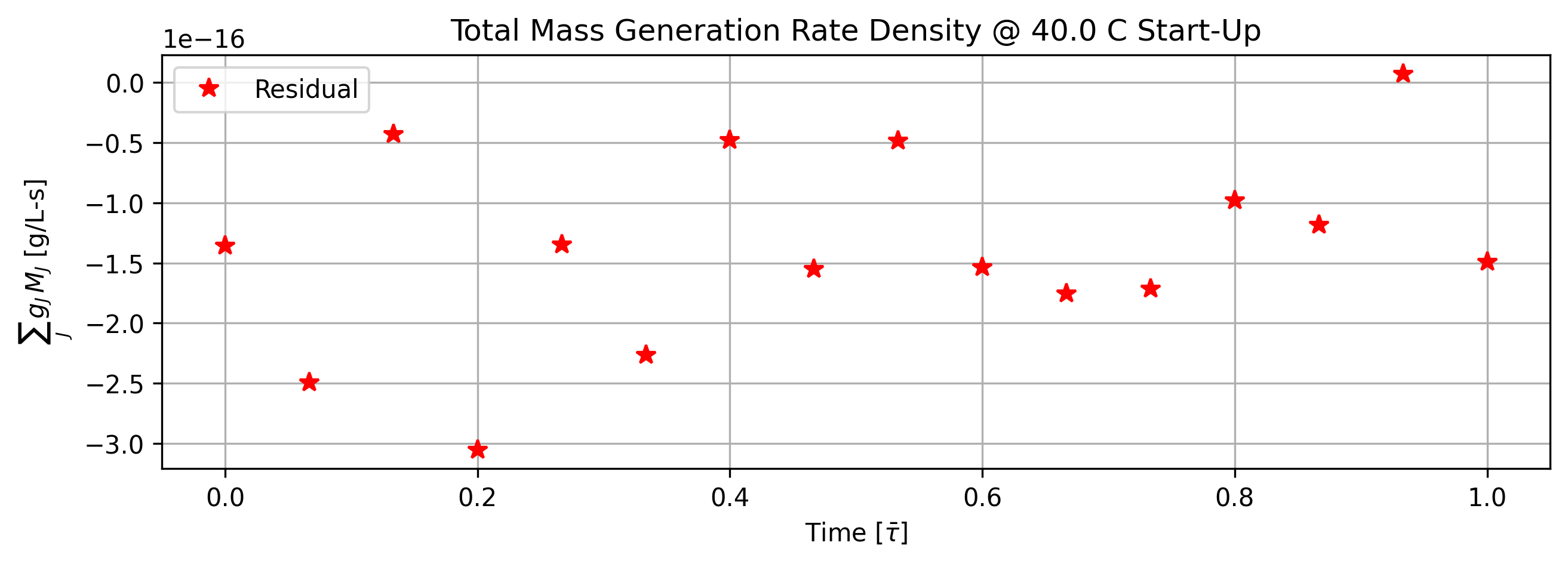
Figure 13: Total mass generation rate density residual history at start-up.

if cortix_ai:
    issues = '+ Title your reponse as: Total Mass Generation Rate Density Residual at Start-Up.'
    cortix_ai.explain(quant=quant, issues=issues, markdown_header_level='<h4>', markdown_display=markdown_display, print_prompt=False, save_supporting_info=db_save)

Cortix AI assistant: working on explanation...

Total Mass Generation Rate Density Residual at Start-Up

Data overview

• The table contains 8 samples of “Total Mass Generation Rate Density [g/L-s]” measured in the mixing volume, paired with time in seconds.

• Time range: 0.00000 s to 48.1638 s, sampled at a constant interval of 6.88054 s (uniform spacing; 7 intervals of 6.88054 s).

Values (quick view)

• Reported density values (g/L-s): -1.36e-16, -4.29886e-17, -1.34644e-16, -4.80098e-17, -4.82605e-17, -1.75336e-16, -9.81881e-17, 7.31159e-18.

• Signs: seven values are negative, one small positive value occurs at the final sample (7.31159e-18).

Statistical summary (units: g/L-s)

• Count: 8 samples.

• Minimum: -1.75336e-16.

• Maximum: 7.31159e-18.

• Mean (average): -8.45e-17.

• Standard deviation (population): 5.74e-17.

• Root-mean-square (RMS): 1.02e-16.

• Maximum absolute residual: 1.75336e-16.

Interpretation

• All values are on the order of 10⁻¹⁶–10⁻¹⁷ g/L-s, i.e., extremely small magnitudes relative to typical engineering scales; the mean and extremes indicate residuals close to numerical zero.

• The time sampling is uniform; there is no sustained drift in the residuals over the recorded interval—values fluctuate around zero with typical dispersion given by the standard deviation above.

• For mass-balance diagnostics, these numbers indicate mass-generation-rate residuals at start-up are effectively negligible within the shown precision.

AI Parameters:
+ LLM model (OpenAI) = gpt-5-mini
+ LLM cleverness     = 1.0
+ Total # of tokens  = 5546

1.6. Steady-State Simulation

Pick up from where it left from the past run() and continue to a longer time. This demonstrates how to continue a simulation from where it was interrupted. Note that the state of the system is automatically used as the initial condition for the next run().

end_time += 5 * stg.flow_residence_time_avg
time_step = 5 * stg.flow_residence_time_avg / 15
show_time = (True, 10*time_step)

stg.time_step = time_step
stg.initial_time = stg.end_time
stg.end_time = end_time
stg.show_time = show_time

'''Run system in parallel'''
stg.monitor_mass_flowrates = False
stg.monitor_mass_conservation_residual = False
system.run()
system.close() # Shutdown Cortix

[31384] 2025-12-02 15:52:35,612 - cortix - INFO - Launching Module <solvex.stage.Stage object at 0x7f85423be5d0>
[910] 2025-12-02 15:52:36,803 - cortix - INFO - Stg-1::run():time[m]=0.9
[910] 2025-12-02 15:52:37,055 - cortix - INFO - Stg-1::run():time[m]=3.7
Total mass rate density (mixture volume) residual [g/L-s]= -2.84061e-17
total mass inflow rate [g/min]   = 6.711e+02
total mass outflow rate [g/min]  =  6.711e+02
	 net total mass flow rate [g/min] = -1.359e-05
[910] 2025-12-02 15:52:37,140 - cortix - INFO - Stg-1::run():time[m]=5.2 (et[s]=0.3)
[31384] 2025-12-02 15:52:37,329 - cortix - INFO - run()::Elapsed wall clock time [s]: 744.99
[31384] 2025-12-02 15:52:37,330 - cortix - INFO - Closed Cortix object.
_____________________________________________________________________________
                           T E R M I N A T I N G                             
_____________________________________________________________________________
      ...                                        s       .     (TAAG Fraktur)
   xH88"`~ .x8X                                 :8      @88>
 :8888   .f"8888Hf        u.      .u    .      .88      %8P      uL   ..
:8888>  X8L  ^""`   ...ue888b   .d88B :@8c    :888ooo    .     .@88b  @88R
X8888  X888h        888R Y888r ="8888f8888r -*8888888  .@88u  ""Y888k/"*P
88888  !88888.      888R I888>   4888>"88"    8888    888E`    Y888L
88888   %88888      888R I888>   4888> "      8888      888E      8888
88888 `> `8888>     888R I888>   4888>        8888      888E      `888N
`8888L %  ?888   ! u8888cJ888   .d888L .+    .8888Lu=   888E   .u./"888&
 `8888  `-*""   /   "*888*P"    ^"8888*"     ^%888*     888&  d888" Y888*"
   "888.      :"      "Y"          "Y"         "Y"      R888" ` "Y   Y"
     `""***~"`                                           ""
                             https://cortix.org                              
_____________________________________________________________________________
[31384] 2025-12-02 15:52:37,331 - cortix - INFO - close()::Elapsed wall clock time [s]: 745.0

'''Recover stage'''
stg = system_net.modules[0]

1.6.1. Organic Phase Results

'''Plot organic phase'''
# TODO: time axis normalized by phase flow residence time.
stg.organic_phase.plot(title='Organic Phase Steady-State', legend='Organic Phase', nrows=2,ncols=3, show=True, figsize=[12,6])

fig_count += 1
print(f'Figure {fig_count}: Organic phase species history dashboard at steady-state.')

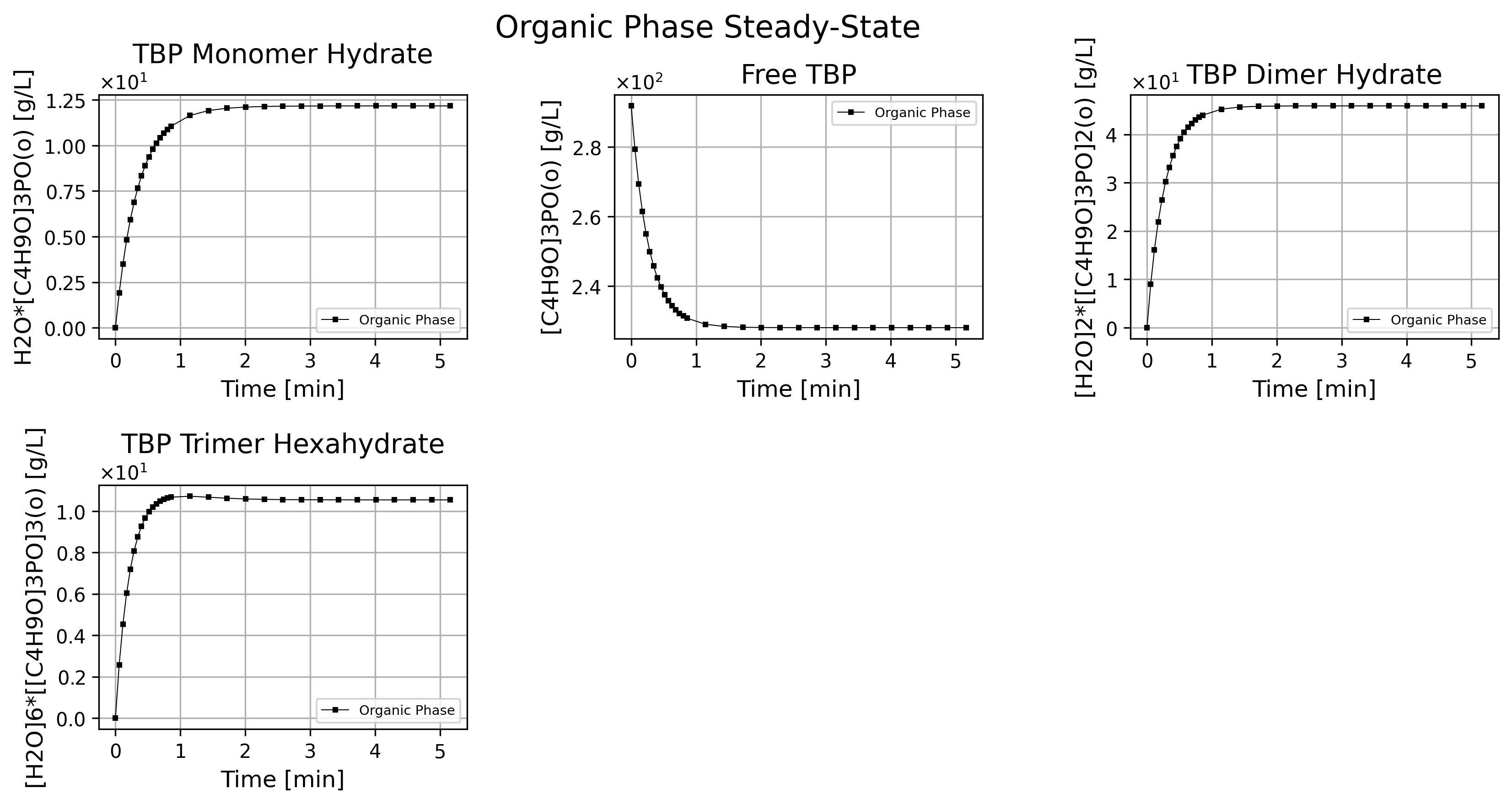
Figure 14: Organic phase species history dashboard at steady-state.

if cortix_ai:
    issues = ('+ Title your reponse as: Overview of the Organic Phase Data at Steady-State.\n'
              '+ Do not explain the start-up process; cover the steady-state only.'
    )
    cortix_ai.explain(phase=stg.organic_phase, markdown_header_level='<h4>', markdown_display=markdown_display, save_supporting_info=db_save)

Cortix AI assistant: working on explanation...

Summary

• The dataset tracks four species over 0–310 s: H₂O·[C₄H₉O]₃PO(o), [C₄H₉O]₃PO(o), [H₂O]₂·[[C₄H₉O]₃PO]₂(o), and [H₂O]₆·[[C₄H₉O]₃PO]₃(o).

• [C₄H₉O]₃PO(o) decreases from 291.750 g/L to 228.085 g/L; the three water‑associated species rise from 0 to steady, with most change occurring before ≈120 s and values approaching a plateau by ≈150 s–200 s.

Column-wise analysis

• [C₄H₉O]₃PO(o): initial 291.750 → final 228.085 g/L; absolute change −63.665 g/L (≈ −21.8%). Rapid decrease in the first ~50 s, then slowing and near‑steady by ~120 s.

• H₂O·[C₄H₉O]₃PO(o): initial 0 → final 12.1757 g/L; monotonic increase, most of the rise occurs in the first ~70 s, then approaches a small steady value (~12.17 g/L).

• [H₂O]₂·[[C₄H₉O]₃PO]₂(o): initial 0 → final 45.8827 g/L; largest absolute accumulation among the formed species, with rapid formation early and a clear plateau by ~120 s.

• [H₂O]₆·[[C₄H₉O]₃PO]₃(o): initial 0 → final 10.5415 g/L; increases quickly at first and then levels off to ≈10.54 g/L.

Comparative observations

• Absolute gains: the dimer [H₂O]₂·[[C₄H₉O]₃PO]₂(o) shows the largest absolute increase (+45.883 g/L), followed by H₂O·[C₄H₉O]₃PO(o) (+12.176 g/L) and [H₂O]₆·[[C₄H₉O]₃PO]₃(o) (+10.542 g/L).

• Largest absolute loss: the monomer [C₄H₉O]₃PO(o) (−63.665 g/L), consistent with its conversion into the three water‑associated species.

• Relative retention: the monomer retains ≈78.2% of its initial concentration at the end (228.085/291.75).

Temporal dynamics

• Two phases are visible: a fast transient (≈0–50–120 s) with most concentration change, and a slow approach to steady state (≈120–310 s) with only minor further changes.

• Example rates (approximate): between 0 and 31 s the monomer drops ≈54.20 g/L (≈1.75 g·L⁻¹·s⁻¹ average over that interval); after ~120 s the changes are <0.05 g/L over hundreds of seconds (negligible compared with the initial transient).

Total across listed species (simple sum) and mass‑balance note

• Sum of the four listed concentrations:

  • t = 0 s: 291.750 g/L

  • t = 3.44 s: 292.745 g/L

  • t = 309.624 s: 296.685 g/L

• The total increases by ≈4.935 g/L (≈ +1.69%) from t = 0 to t = 309.6 s. The dataset therefore does not show strict conservation of the simple sum of these four columns (the summed quantity rises and then plateaus), which is evident from the numbers above.

Concise conclusions

• The system converts a significant fraction (~21.8%) of [C₄H₉O]₃PO(o) into water‑associated complexes, predominantly forming the dimeric complex [H₂O]₂·[[C₄H₉O]₃PO]₂(o).

• Most conversion occurs within the first ~100–150 s, after which all four concentrations are effectively at steady values within the provided precision.

AI Parameters:
+ LLM model (OpenAI) = gpt-5-mini
+ LLM cleverness     = 1.0
+ Total # of tokens  = 6345

'''Compute molar concentration of TBP species'''
import numpy as np

tbp_mass_cc_org_history = stg.organic_phase.get_column(tbp_org_name)
tbp_molar_cc_org_history = np.array(tbp_mass_cc_org_history)/tbp_org.molar_mass

tbp_monomer_mass_cc_org_history = stg.organic_phase.get_column(tbp_monomer_org_name)
tbp_monomer_molar_cc_org_history = np.array(tbp_monomer_mass_cc_org_history)/tbp_monomer_org.molar_mass

tbp_dimer_mass_cc_org_history = stg.organic_phase.get_column(tbp_dimer_org_name)
tbp_dimer_molar_cc_org_history = np.array(tbp_dimer_mass_cc_org_history)/tbp_dimer_org.molar_mass

tbp_trimer_hexahydrate_mass_cc_org_history = stg.organic_phase.get_column(tbp_trimer_hexahydrate_org_name)
tbp_trimer_hexahydrate_molar_cc_org_history = np.array(tbp_trimer_hexahydrate_mass_cc_org_history)/tbp_trimer_hexahydrate_org.molar_mass

time_stamps = np.array(stg.organic_phase.time_stamps)

tbl_count += 1
print(f'Table {tbl_count}: Molarity history of TBP in the organic phase at steady-state.')
print('Time [min] | Free TBP [M] | TBP Monomer [M] | TBP Dimer [M] | TBP Trimer Hexahydrate [M] | balance |')
np.set_printoptions(precision=3, suppress=True, linewidth=100)
for t,a,b,c,d in zip(time_stamps[n_startup::5]/unit.min, 
                     tbp_molar_cc_org_history[n_startup::5]/unit.molar, 
                     tbp_monomer_molar_cc_org_history[n_startup::5]/unit.molar, 
                     tbp_dimer_molar_cc_org_history[n_startup::5]/unit.molar, 
                     tbp_trimer_hexahydrate_molar_cc_org_history[n_startup::5]/unit.molar):
    balance = a+b+2*c+3*d - tbp_mass_cc_org/tbp_org.molar_mass/unit.molar
    print('  %1.2e      %1.3f         %1.3e         %1.3e             %1.3e           %+1.2e'%(t, a, b, c, d, balance))

Table 12: Molarity history of TBP in the organic phase at steady-state.
Time [min] | Free TBP [M] | TBP Monomer [M] | TBP Dimer [M] | TBP Trimer Hexahydrate [M] | balance |
  1.15e+00      0.860         4.097e-02         7.950e-02             1.182e-02           +4.44e-16
  2.58e+00      0.856         4.277e-02         8.068e-02             1.164e-02           +2.22e-16
  4.01e+00      0.856         4.282e-02         8.069e-02             1.162e-02           +4.44e-16

'''Volume fraction of TBP at start-up'''
tbl_count += 1
print(f'Table {tbl_count}: Volume fractions of free and total TBP in the organic phase at steady-state.')
print('Time [min] | Free TBP vol frac [%] | Total TBP vol frac [%] |')
np.set_printoptions(precision=3, suppress=True, linewidth=100)
total_tbp_molar_cc_org_history = tbp_molar_cc_org_history + tbp_monomer_molar_cc_org_history + \
                                 2*tbp_dimer_molar_cc_org_history + 3*tbp_trimer_hexahydrate_molar_cc_org_history
total_tbp_mass_cc_org_history = total_tbp_molar_cc_org_history * tbp_org.molar_mass
for t,a,b in zip(time_stamps[::5]/unit.min, 
               np.array(tbp_mass_cc_org_history[::5])/rho_tbp*100, total_tbp_mass_cc_org_history[::5]/rho_tbp*100):
    print('  %1.2e         %1.3f                  %1.3f'%(t, a, b))

Table 13: Volume fractions of free and total TBP in the organic phase at steady-state.
Time [min] | Free TBP vol frac [%] | Total TBP vol frac [%] |
  0.00e+00         30.000                  30.000
  2.87e-01         25.701                  30.000
  5.73e-01         24.244                  30.000
  8.60e-01         23.734                  30.000
  2.29e+00         23.455                  30.000
  3.73e+00         23.453                  30.000
  5.16e+00         23.453                  30.000

'''Total water extracted'''
water_molar_cc_org_history = tbp_monomer_molar_cc_org_history \
                           + 2*tbp_dimer_molar_cc_org_history \
                           + 6*tbp_trimer_hexahydrate_molar_cc_org_history

water_mass_cc_org_history = water_molar_cc_org_history * h2o_aqu.molar_mass

tbl_count += 1
print(f'Table {tbl_count}: Mass concentration and molarity history of water in the organic phase at steady-state.')
print('Time [s] |   [M]   |  [g/L]  |')
np.set_printoptions(precision=3, suppress=True, linewidth=100)
for a,b,c in zip(time_stamps[n_startup::5], water_molar_cc_org_history[n_startup::5]/unit.molar, water_mass_cc_org_history[n_startup::5]):
    print('%1.2e  %1.3e %1.3e'%(a, b, c))

Table 14: Mass concentration and molarity history of water in the organic phase at steady-state.
Time [s] |   [M]   |  [g/L]  |
6.88e+01  2.709e-01 4.880e+00
1.55e+02  2.739e-01 4.935e+00
2.41e+02  2.739e-01 4.935e+00

'''Organic phase mass density'''
import matplotlib.pyplot as plt

quant = stg.mass_density_history('organic')

quant.plot(title='Organic Phase Mass Density @ %2.1f C Steady-State'%unit.convert_temperature(stg_temperature,
           'K','C'), x_scaling=1/stg.flow_residence_time_avg, x_label=r'Time [$\bar{\tau}$]', y_label=quant.latex_name+r'$-\rho_\text{diluent}$'
           ' ['+quant.unit+']', show=True, figsize=[10,3], error_data=False)

fig_count += 1
print(f'Figure {fig_count}: Organic phase mass density history at steady-state.')

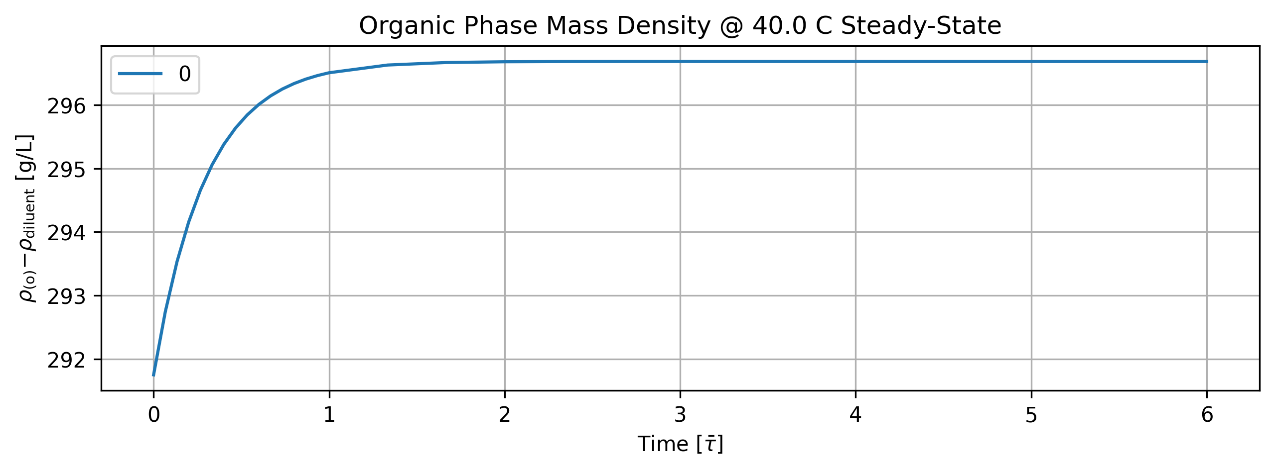
Figure 15: Organic phase mass density history at steady-state.

tbl_count += 1
print(f'Table {tbl_count}: Organic phase mass density history at steady-state.')
print('Time [s]  Organic Phase Mass Density [g/L]')
print(quant.value[::5].apply(lambda x: round(x,2)))

Table 15: Organic phase mass density history at steady-state.
Time [s]  Organic Phase Mass Density [g/L]
0.000000      291.75
17.201342     295.06
34.402683     296.14
51.604025     296.51
137.610734    296.69
223.617442    296.68
309.624151    296.68
Name: Organic Phase Mass Density [g/L]; Time History in [s], dtype: float64

1.6.2. Aqueous Phase Results

'''Plot aqueous phase'''
# TODO: time axis normalized by phase flow residence time.
stg.aqueous_phase.plot(title='Aqueous Phase Steady-State', legend='Aqueous Phase', nrows=2,ncols=3, show=True, figsize=[12,6])

fig_count += 1
print(f'Figure {fig_count}: Aqueous phase species history dashboard at steady-state.')

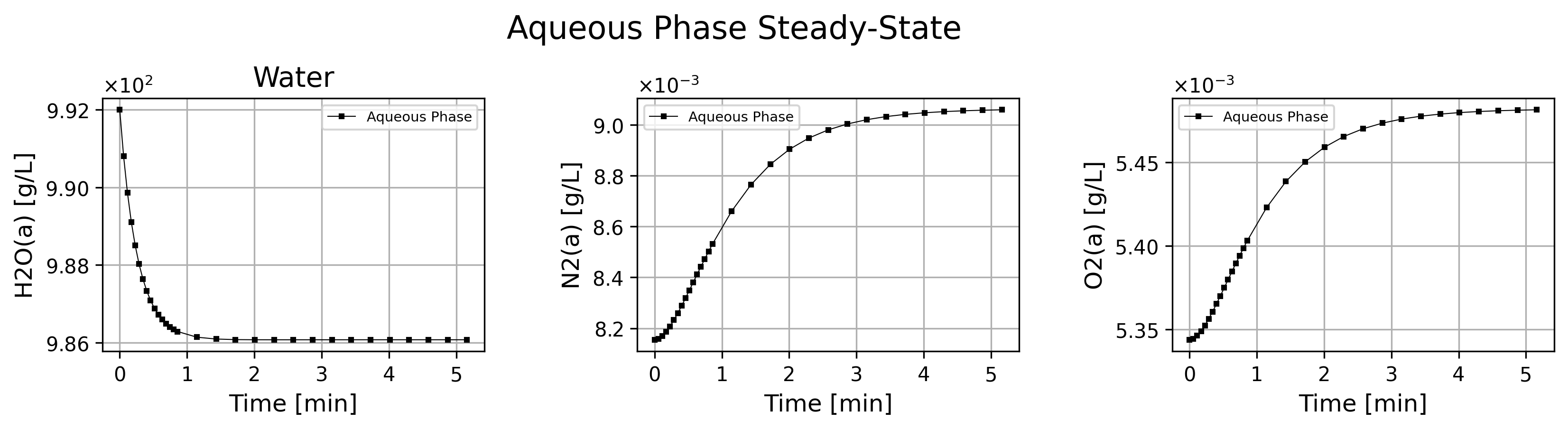
Figure 16: Aqueous phase species history dashboard at steady-state.

if cortix_ai:
    issues = ('+ Title your reponse as: Overview of the Aqueous Phase Data at Steady-State.\n'
              '+ Do not explain the start-up process; cover the steady-state only.'
    )
    cortix_ai.explain(phase=stg.aqueous_phase, markdown_header_level='<h4>', markdown_display=markdown_display, print_prompt=False, save_supporting_info=db_save)

Cortix AI assistant: working on explanation...

Summary

The table reports concentrations (g/L) of H₂O(a), N₂(a), and O₂(a) measured from 0 to 309.624 s; H₂O decreases noticeably while the dissolved gases increase slightly.

• Measurement span: 0 s → 309.624 s.

• H₂O(a) falls from 992 g/L to 986.075 g/L (absolute change −5.925 g/L).

• N₂(a) rises from 0.00815443 g/L to 0.00905861 g/L (absolute change +0.00090418 g/L).

• O₂(a) rises from 0.0053437 g/L to 0.00548158 g/L (absolute change +0.00013788 g/L).

Numerical rates and relative changes

• H₂O(a): average rate ≈ −0.01914 g·L⁻¹·s⁻¹, relative change ≈ −0.597%.

• N₂(a): average rate ≈ +2.92×10⁻⁶ g·L⁻¹·s⁻¹, relative change ≈ +11.1%.

• O₂(a): average rate ≈ +4.45×10⁻⁷ g·L⁻¹·s⁻¹, relative change ≈ +2.58%.

Temporal behavior and steady state

• Early transient (0 → ~30 s): H₂O(a) falls faster in the first few seconds (e.g., −1.193 g/L in the first 3.44 s), then the rate slows.

• Later times (>~100 s): all three concentrations effectively level off; H₂O(a) reaches ≈986.075 g/L and N₂(a), O₂(a) approach ≈0.00906 g/L and ≈0.00548 g/L respectively, showing a near steady state by ~100–140 s.

Comparative magnitudes

• H₂O(a) dominates by five orders of magnitude: H₂O/N₂ ≈ 1.09×10⁵ and H₂O/O₂ ≈ 1.80×10⁵ (using final values).

• N₂(a)/O₂(a) ≈ 1.65 (final values), so N₂(a) is ≈65% higher than O₂(a) in mass concentration.

• Absolute changes in gases are tiny compared with the water concentration; the largest fractional change is for N₂(a) (~11%) because its baseline is very small.

Notes on precision

• Many later rows show values repeating to the displayed precision (e.g., H₂O ≈ 986.075), indicating approach to numerical/experimental steady values or measurement rounding at the reported significant figures.

AI Parameters:
+ LLM model (OpenAI) = gpt-5-mini
+ LLM cleverness     = 1.0
+ Total # of tokens  = 5633

'''Aqueous phase mass density'''
import matplotlib.pyplot as plt

quant = stg.mass_density_history('aqueous')

quant.plot(title='Aqueous Phase Mass Density @ %2.1f C Steady-State'%unit.convert_temperature(stg_temperature,
           'K','C'), x_scaling=1/stg.flow_residence_time_avg, x_label=r'Time [$\bar{\tau}$]', y_label=quant.latex_name+
           ' ['+quant.unit+']', show=True, figsize=[10,3], error_data=False)

fig_count += 1
print(f'Figure {fig_count}: Aqueous phase mass density history at Steady-State.')

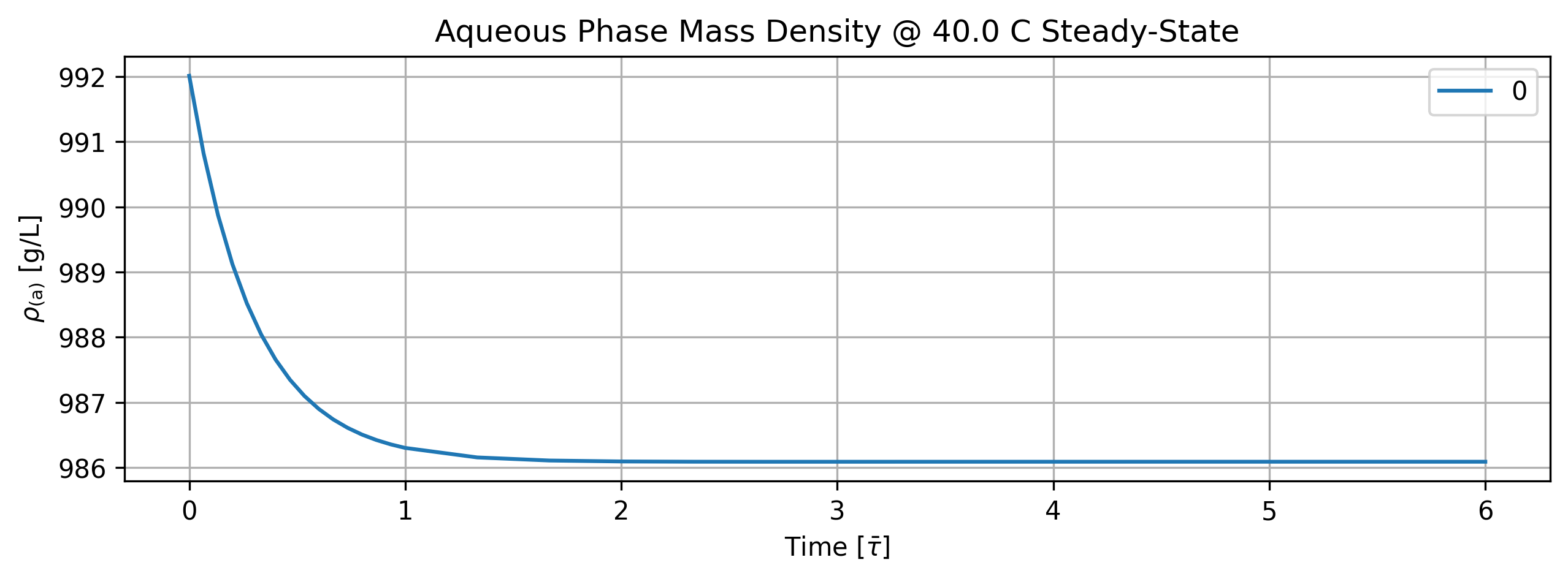
Figure 17: Aqueous phase mass density history at Steady-State.

tbl_count += 1
print(f'Table {tbl_count}: Aqueous phase mass density history at steady-state.')
print('Time [s]  Aqueous Phase Mass Density [g/L]')
print(quant.value[::5].apply(lambda x: round(x,2)))

Table 16: Aqueous phase mass density history at steady-state.
Time [s]  Aqueous Phase Mass Density [g/L]
0.000000      992.01
17.201342     988.04
34.402683     986.74
51.604025     986.30
137.610734    986.09
223.617442    986.09
309.624151    986.09
Name: Aqueous Phase Mass Density [g/L]; Time History in [s], dtype: float64

1.6.3. Vapor Phase Results

'''Plot vapor phase'''
# TODO: time axis normalized by phase flow residence time.
stg.vapor_phase.plot(title='Vapor Phase Steady-State', legend='Vapor Phase', nrows=2,ncols=3, show=True, figsize=[12,6])

fig_count += 1
print(f'Figure {fig_count}: Vapor phase species history dashboard at steady-state.')

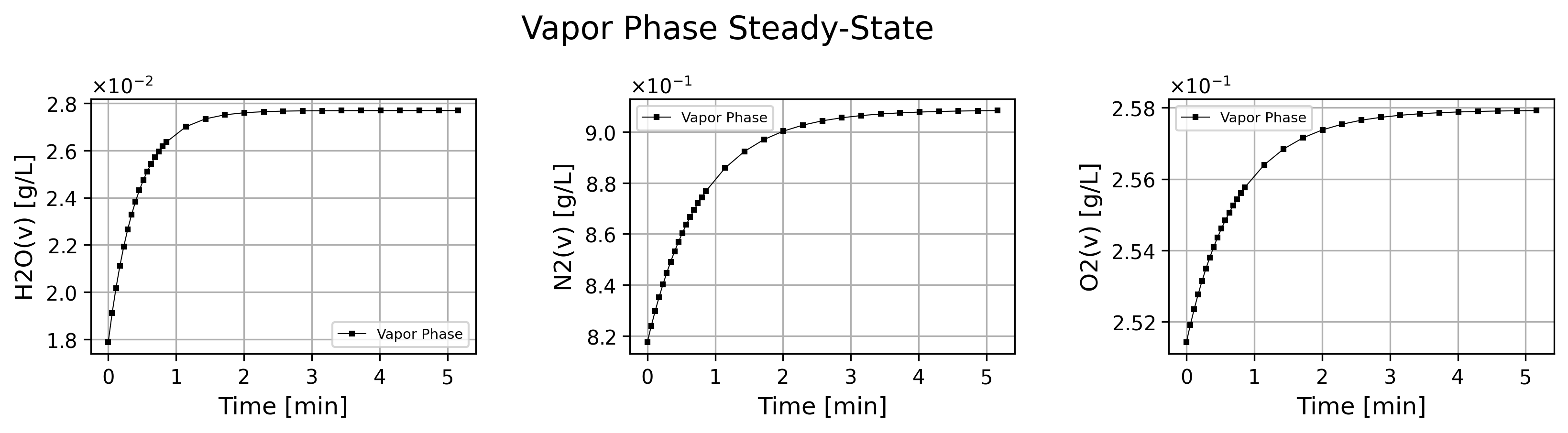
Figure 18: Vapor phase species history dashboard at steady-state.

if cortix_ai:
    issues = ('+ Title your reponse as: Overview of the Vapor Phase Data at Steady-State.\n'
              '+ Do not explain the start-up process; cover the steady-state only.'
    )
    cortix_ai.explain(phase=stg.vapor_phase, issues=issues, markdown_header_level='<h4>', markdown_display=markdown_display, save_supporting_info=db_save)

Cortix AI assistant: working on explanation...

Overview of the Vapor Phase Data at Steady-State.

Steady-state window

• Time window analyzed: from 120.409 s to 309.624 s (12 data points).

• Focus: concentrations in the vapor phase for H₂O(v), N₂(v), and O₂(v) within that window.

Numerical summary (steady-state)

• H₂O(v)

  • Mean concentration: 0.0276814 g/L

  • Minimum: 0.0276049 g/L; Maximum: 0.0276972 g/L

  • Absolute range: 9.23 × 10⁻⁵ g/L

  • Change from first to last steady point: +0.0000923 g/L (+0.33%)

• N₂(v)

  • Mean concentration: 0.9062283 g/L

  • Minimum: 0.900343 g/L; Maximum: 0.908398 g/L

  • Absolute range: 0.008055 g/L

  • Change from first to last steady point: +0.008055 g/L (+0.89%)

• O₂(v)

  • Mean concentration: 0.2577753 g/L

  • Minimum: 0.257380 g/L; Maximum: 0.257921 g/L

  • Absolute range: 0.000541 g/L

  • Change from first to last steady point: +0.000541 g/L (+0.21%)

Comparative observations

• Abundance ranking (by mean concentration): N₂(v) >> O₂(v) >> H₂O(v).

  • Mean ratios: N₂/O₂ ≈ 3.52; N₂/H₂O ≈ 32.7; O₂/H₂O ≈ 9.31.

• Stability (relative change over steady window):

  • O₂(v) and H₂O(v) show very small relative changes (≈0.21% and ≈0.33%, respectively).

  • N₂(v) shows the largest relative drift within the steady window (≈0.89%), though absolute concentration remains ~0.9 g/L.

• Absolute variability:

  • N₂(v) has the largest absolute range (8.06 × 10⁻³ g/L), driven by its larger base concentration.

  • H₂O(v) and O₂(v) vary only by 10⁻⁴–10⁻³ g/L in absolute terms.

Conclusions

• Over the selected steady-state window (120.4–309.6 s) the vapor-phase concentrations are effectively constant to within sub-percent changes.

• N₂(v) dominates by mass and shows the largest absolute and relative drift in this interval; O₂(v) and H₂O(v) are comparatively stable with sub‑0.4% changes.

AI Parameters:
+ LLM model (OpenAI) = gpt-5-mini
+ LLM cleverness     = 1.0
+ Total # of tokens  = 6897

'''Vapor phase mass density'''
import matplotlib.pyplot as plt

quant = stg.mass_density_history('vapor')

quant.plot(title='Vapor Phase Mass Density @ %2.1f C Steady-State'%unit.convert_temperature(stg_temperature,
           'K','C'), x_scaling=1/stg.flow_residence_time_avg, x_label=r'Time [$\bar{\tau}$]', y_label=quant.latex_name+
           ' ['+quant.unit+']', show=True, figsize=[10,3], error_data=False)

fig_count += 1
print(f'Figure {fig_count}: Vapor phase mass density history at steady-state.')

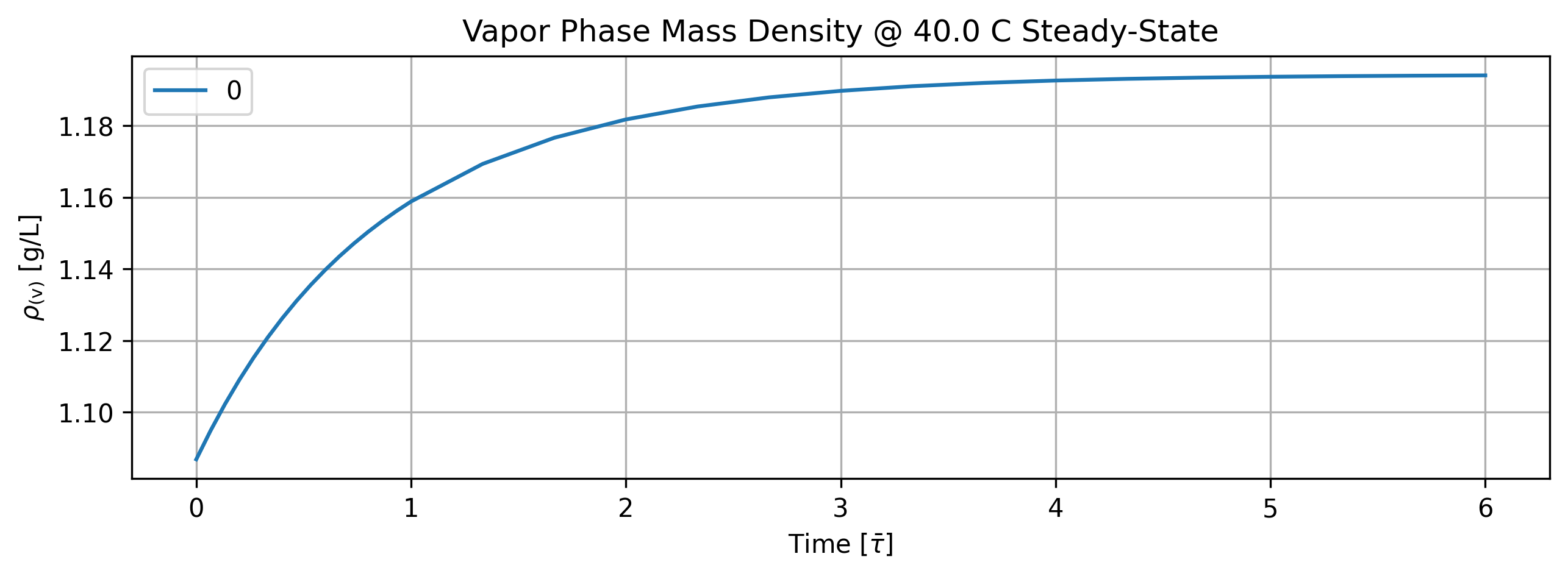
Figure 19: Vapor phase mass density history at steady-state.

tbl_count += 1
print(f'Table {tbl_count}: Vapor phase mass density history at steady-state.')
print('Time [s]  Vapor Phase Mass Density [g/L]')
print(quant.value[::5].apply(lambda x: round(x,2)))

Table 17: Vapor phase mass density history at steady-state.
Time [s]  Vapor Phase Mass Density [g/L]
0.000000      1.09
17.201342     1.12
34.402683     1.14
51.604025     1.16
137.610734    1.19
223.617442    1.19
309.624151    1.19
Name: Vapor Phase Mass Density [g/L]; Time History in [s], dtype: float64

1.6.3.1. Relative Humidity

'''Compute relative humidity in the vapor phase'''
import matplotlib.pyplot as plt
from solvex import air_relative_humidity
from copy import deepcopy

h2o_vap_pd_series = deepcopy(stg.vapor_phase.df['H2O(v)'])
for idx, rho_h2o in enumerate(h2o_vap_pd_series):
    h2o_vap_pd_series.iloc[idx] = air_relative_humidity(stg_temperature, rho_h2o)
rh_pd_series = h2o_vap_pd_series
time_unit = stg.vapor_phase.time_unit
rh_pd_series.name = f'Relative Humidity History [{time_unit}]'
  
quant = Quantity(name=rh_pd_series.name, latex_name='RH', unit='%', info=f'Relative Humidity History (Vapor Phase) [{time_unit}]')
quant.value = h2o_vap_pd_series
quant.plot(title='Stage Rel. Humidity @ %2.1f C Steady-State'%unit.convert_temperature(stg_temperature, 'K','C'),
           x_scaling=1/stg.flow_residence_time_avg, x_label=r'Time [$\bar{\tau}$]', y_label=quant.latex_name+' ['+quant.unit+']', show=True, 
           figsize=[10,3])

fig_count += 1
print(f'Figure {fig_count}: Stage relative humidity history at steady-state.')

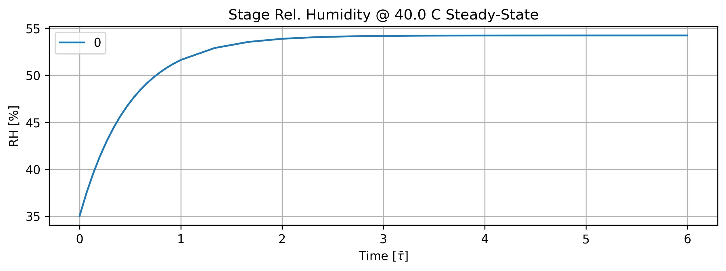
Figure 20: Stage relative humidity history at steady-state.

tbl_count += 1
print(f'Table {tbl_count}: Stage relative humidity history at steady-state.')
print('Time [s]  Rel. Humidity [%]')
print(quant.value.loc[n_startup::5].apply(lambda x: round(x,2)))

Table 18: Stage relative humidity history at steady-state.
Time [s]  Rel. Humidity [%]
17.201342     44.36
34.402683     49.16
51.604025     51.63
137.610734    54.14
223.617442    54.23
309.624151    54.23
Name: Relative Humidity History [s], dtype: float64

if cortix_ai:
    issues = ('+ Title your reponse as: Overview of the Relative Humidity Data at Steady-State.\n'
              '+ Do not explain the start-up process; cover the steady-state only.'
    )
    cortix_ai.explain(quant=quant, issues=issues, markdown_header_level='<h5>', markdown_display=markdown_display, print_prompt=False, save_supporting_info=db_save)

Cortix AI assistant: working on explanation...

Overview of the Relative Humidity Data at Steady-State.

Steady-state is taken from the portion of the table where RH values are effectively constant (the last four rows).

Steady-state time window

• Indices used: 7–10 (time = 154.812 s, 206.416 s, 258.02 s, 309.624 s).

• Measured quantity: Relative Humidity (third column) expressed in % and sampled at the times given in seconds.

Statistical summary (indices 7–10)

• Sample size: n = 4.

• Mean RH: 54.217% (arithmetic mean of 54.1827, 54.2239, 54.2295, 54.2303).

• Minimum RH: 54.1827%.

• Maximum RH: 54.2303%.

• Absolute range: 0.0476 percentage points.

• Population standard deviation: ≈ 0.0197% (sample standard deviation ≈ 0.0228%).

• Coefficient of variation: ≈ 0.036% (std/mean × 100).

Sampling and short-term trend within steady-state

• Sampling interval between steady-state points: constant 51.604 s (exact spacing between consecutive times).

• Linear change over the window (154.812 s -> 309.624 s): RH increases by 0.0476 percentage points, giving a slope ≈ 0.0003076 %/s (≈ 0.0308% per 100 s).

• Fluctuation magnitude in this window is very small (≤ 0.05 percentage points), indicating tight clustering around the mean.

Concise interpretation

• The RH has reached a stable level near 54.22% with very small absolute fluctuations (range 0.0476% and population std ≈ 0.02%), sampled at regular 51.604 s intervals. The residual drift over the analyzed window is ≈ 0.00031 %/s, so values can be treated as steady within typical measurement precision.

AI Parameters:
+ LLM model (OpenAI) = gpt-5-mini
+ LLM cleverness     = 1.0
+ Total # of tokens  = 4613

1.6.4. Overall Stage Efficiency

'''Stage overall efficiency'''

quant = stg.efficiency_history(mean=True)
quant.plot(title='Stage Efficiency @ %2.1f C Steady-State'%unit.convert_temperature(stg_temperature,
           'K','C'), x_scaling=1/stg.flow_residence_time_avg, x_label=r'Time [$\bar{\tau}$]', y_label=quant.latex_name+
           ' ['+quant.unit+']', show=True, figsize=[10,3], error_data=True)

fig_count += 1
print(f'Figure {fig_count}: Stage efficiency history steady-state.')

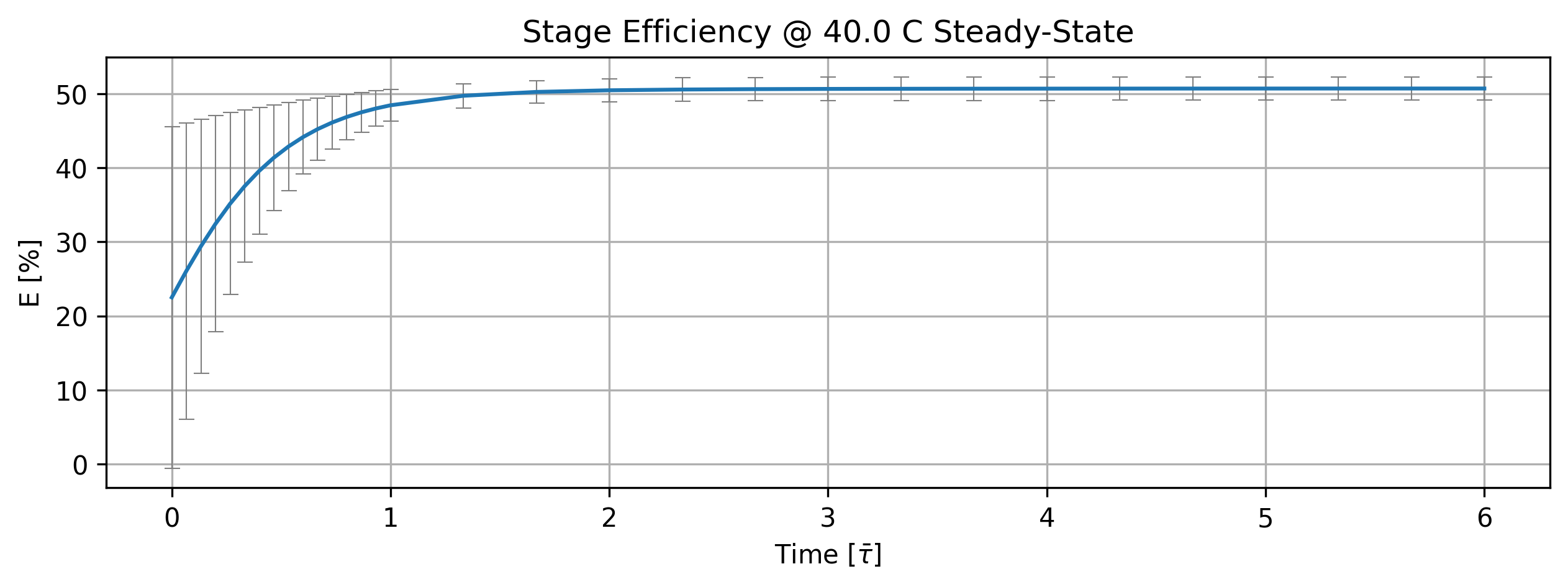
Figure 21: Stage efficiency history steady-state.

tbl_count += 1
print(f'Table {tbl_count}: Stage efficiency history at steady-state.')
print('Time [s]  (Stage. Eff., +-std) [%]')
time_name = ''
import pandas as pd
df = (quant.value.apply(pd.Series).mul(1)
       .rename(index=lambda i: round(i/unit.min,2))
       .set_axis(['',''], axis=1).rename_axis(time_name)
       .round(3))
print(df.to_string(max_rows=20, min_rows=20))

Table 19: Stage efficiency history at steady-state.
Time [s]  (Stage. Eff., +-std) [%]
                    
                    
0.00  22.500  23.049
0.06  26.079  20.002
0.11  29.411  17.158
0.17  32.443  14.575
0.23  35.149  12.284
0.29  37.528  10.291
0.34  39.592   8.587
0.40  41.363   7.153
0.46  42.871   5.962
0.52  44.146   4.984
...      ...     ...
2.58  50.649   1.583
2.87  50.667   1.584
3.15  50.679   1.584
3.44  50.687   1.582
3.73  50.692   1.581
4.01  50.696   1.580
4.30  50.699   1.579
4.59  50.700   1.579
4.87  50.702   1.578
5.16  50.703   1.578

if cortix_ai:
    issues = ('+ Title your reponse as: Overview of the Stage Efficiency Data at Steady-State.\n'
              '+ Do not explain the start-up process; cover the steady-state only.'
    )
    cortix_ai.explain(quant=quant, issues=issues, markdown_header_level='<h4>', markdown_display=markdown_display, save_supporting_info=db_save)

Cortix AI assistant: working on explanation...

Overview of the Stage Efficiency Data at Steady-State.

• Steady-state interval selected: t ≥ 103.208 s (rows 6–10 in the table).

• Time column (steady-state window):

  • Range: 103.208 s to 309.624 s.

  • Sampling: nonuniform times; final four samples are ≈51.604 s apart.

• Mean efficiency (column “0”) in steady state:

  • Values: 50.4626, 50.6486, 50.6866, 50.6986, 50.7027 [%].

  • Average (mean over steady-state samples): ≈ 50.64 [%].

  • Temporal spread: min = 50.4626 [%], max = 50.7027 [%], range = 0.2401 percentage points.

  • Temporal variability (standard deviation of these five values): ≈ 0.10 percentage points (≈0.2% relative to the mean).

• Reported uncertainty (column “1”, the ±std values) in steady state:

  • Values: 1.55553, 1.58311, 1.58244, 1.57935, 1.57778 [%].

  • Mean reported std: ≈ 1.576 [%].

  • Variation of reported std across the window: min = 1.55553 [%], max = 1.58311 [%], range ≈ 0.0276 percentage points; std ≈ 0.01 percentage points.

• Interpretation (steady-state only):

  • The stage operates at an average efficiency of ≈ 50.64% with a per-sample uncertainty of about ±1.576 percentage points.

  • The temporal drift/fluctuation of the mean efficiency within the chosen steady-state window (≈0.10 ppt) is small compared with the reported per-sample standard deviation (≈1.576 ppt), i.e., temporal changes are negligible relative to measurement/spread.

AI Parameters:
+ LLM model (OpenAI) = gpt-5-mini
+ LLM cleverness     = 1.0
+ Total # of tokens  = 5353

'''Individual reaction efficiency'''

quant = stg.efficiency_history()
quant.plot(title='Reaction Efficiency @ %2.1f C Steady-State'%unit.convert_temperature(stg_temperature,
           'K','C'), x_scaling=1/stg.flow_residence_time_avg, x_label=r'Time [$\bar{\tau}$]', y_label=quant.latex_name+
           ' ['+quant.unit+']', legend=stg.rxn_mech.reactions, show=True, figsize=[10,3])

fig_count += 1
print(f'Figure {fig_count}: Reaction efficiency history at steady-state.')

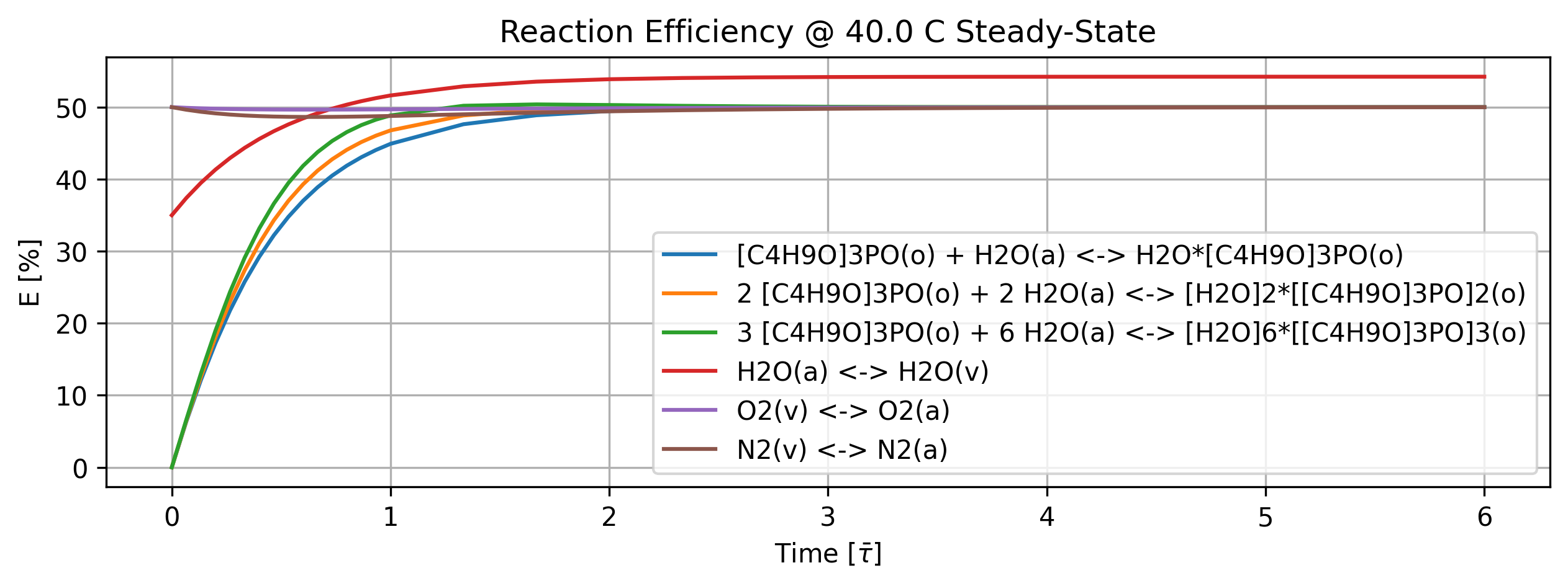
Figure 22: Reaction efficiency history at steady-state.

'''Individual reaction efficiency'''
quant = stg.efficiency_history()
tbl_count += 1
print(f'Table {tbl_count}: Reaction efficiency history at steady-state.')
print('Time [min]    Rxn Eff. [%]')

col_names = [f'r{i}' for i in range(len(stg.rxn_mech.reactions))]
time_name = ''
df = (quant.value.apply(pd.Series).mul(1)
       .rename(index=lambda i: round(i/unit.min,2))
       .set_axis(col_names, axis=1).rename_axis(time_name)
       .round(3))
print(df.to_string(max_rows=20, min_rows=20))

Table 20: Reaction efficiency history at steady-state.
Time [min]    Rxn Eff. [%]
          r0      r1      r2      r3      r4      r5
                                                    
0.00   0.000   0.000   0.000  35.000  50.000  50.000
0.06   6.372   6.506   6.644  37.401  49.910  49.642
0.11  12.131  12.581  13.054  39.502  49.839  49.359
0.17  17.270  18.111  19.012  41.340  49.783  49.140
0.23  21.807  23.042  24.383  42.949  49.741  48.972
0.29  25.779  27.366  29.107  44.358  49.710  48.847
0.34  29.232  31.105  33.176  45.590  49.688  48.758
0.40  32.218  34.303  36.618  46.669  49.674  48.698
0.46  34.790  37.011  39.488  47.613  49.665  48.661
0.52  36.997  39.288  41.849  48.439  49.661  48.644
...      ...     ...     ...     ...     ...     ...
2.58  49.933  49.995  50.061  54.183  49.946  49.774
2.87  49.966  49.998  50.033  54.206  49.961  49.836
3.15  49.983  50.000  50.018  54.218  49.972  49.882
3.44  49.991  50.000  50.009  54.224  49.980  49.915
3.73  49.996  50.000  50.005  54.228  49.986  49.939
4.01  49.998  50.000  50.002  54.229  49.990  49.956
4.30  49.999  50.000  50.001  54.230  49.993  49.969
4.59  49.999  50.000  50.001  54.230  49.995  49.978
4.87  50.000  50.000  50.000  54.231  49.996  49.984
5.16  50.000  50.000  50.000  54.231  49.997  49.988

if cortix_ai:
    issues = ('+ Title your reponse as: Overview of Individual Reaction Efficiency at Steady-State'
             '+ Do not explain the start-up process; cover the steady-state only.'
    )
    cortix_ai.explain(quant=quant, issues=issues, markdown_header_level='<h4>', markdown_display=markdown_display, save_supporting_info=db_save)

Cortix AI assistant: working on explanation...

Overview of Individual Reaction Efficiency at Steady-State+

Steady-state window and overall observation

• Steady-state assessed from the final five time points (time = 103.208 s through 309.624 s). All six reactions settle to nearly constant efficiencies over that window: five reactions cluster very close to 50% and one reaction is consistently higher ≈54.15%.

Per-reaction steady-state statistics (rows 6–10)

• Reaction 1 — [C₄H₉O]₃PO(o) + H₂O(a) <=> H₂O·[C₄H₉O]₃PO(o): mean = 49.876% ; observed range = 49.4555 → 49.9998 (Δ = 0.544 percentage points; ±~1.09% relative to mean).

• Reaction 2 — 2 [C₄H₉O]₃PO(o) + 2 H₂O(a) <=> [H₂O]₂·[[C₄H₉O]₃PO]₂(o): mean = 49.971% ; observed range = 49.8587 → 50.0000 (Δ = 0.141 percentage points; ±~0.28% relative).

• Reaction 3 — 3 [C₄H₉O]₃PO(o) + 6 H₂O(a) <=> [H₂O]₆·[[C₄H₉O]₃PO]₃(o): mean = 50.074% ; observed range = 50.0002 → 50.2991 (Δ = 0.299 percentage points; ±~0.60% relative).

• Reaction 4 — H₂O(a) <=> H₂O(v): mean = 54.149% ; observed range = 53.8787 → 54.2308 (Δ = 0.352 percentage points; ±~0.65% relative). This reaction is the only one with a steady-state mean noticeably above 50%.

• Reaction 5 — O₂(v) <=> O₂(a): mean = 49.955% ; observed range = 49.8605 → 49.9973 (Δ = 0.137 percentage points; ±~0.27% relative).

• Reaction 6 — N₂(v) <=> N₂(a): mean = 49.814% ; observed range = 49.4232 → 49.9884 (Δ = 0.565 percentage points; ±~1.14% relative).

Concise interpretation

• By the chosen steady-state window, efficiencies are effectively stabilized: low absolute ranges (≤ ~0.6 percentage points for most reactions, up to ~0.56 for two) indicate small residual variability.

• Except for H₂O(a) <=> H₂O(v) (Reaction 4) at ≈54.15%, all reactions converge to values very close to 50%.

AI Parameters:
+ LLM model (OpenAI) = gpt-5-mini
+ LLM cleverness     = 1.0
+ Total # of tokens  = 6322

1.6.4.1. Total water extracted in equilibrium

From reference: 1994 Naganawa and Tachimori Anal. Sci. 10 p 607

[H2O]_o,E = 0.4265 M

Comparison to steady state:

h2o_e_molar = water_molar_cc_org_history[-1]/unit.molar

print('Total H2O extracted [M] = %1.4f'%h2o_e_molar)
print('Error (compared to measurement) [%%] = %1.2f'%((h2o_e_molar-0.4265)/0.4265*100))

Total H2O extracted [M] = 0.2739
Error (compared to measurement) [%] = -35.77

1.6.5. Reaction Rate Density

This quantity only makes sense per volume of the mixture.

'''Reaction rate density'''
import matplotlib.pyplot as plt

quant = stg.r_vec_history()# mole/m^3-s

quant.plot(title='Reaction Rate Density @ %2.1f C Steady-State'%unit.convert_temperature(stg_temperature,
           'K','C'), x_scaling=1/stg.flow_residence_time_avg, x_label=r'Time [$\bar{\tau}$]', y_label=quant.latex_name+
           ' ['+quant.unit+']', legend=stg.rxn_mech.reactions, show=True, figsize=[10,3], error_data=False)

fig_count += 1
print(f'Figure {fig_count}: Reaction rate density history at steady-state.')

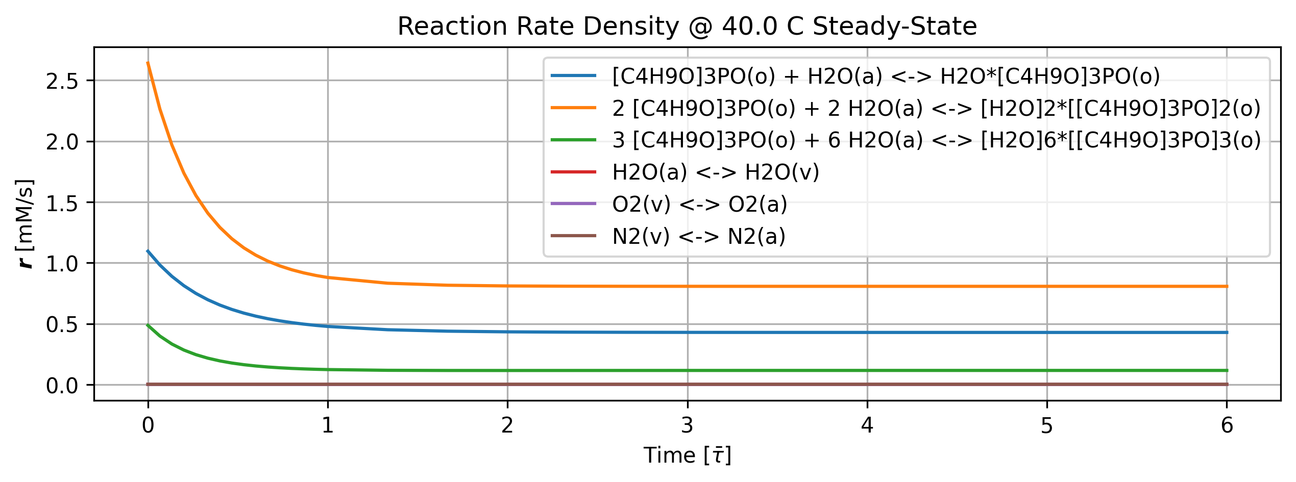
Figure 23: Reaction rate density history at steady-state.

tbl_count += 1
print(f'Table {tbl_count}: Reaction rate density history at steady-state.')
print('Time [min]      r [mM/s]')
import pandas as pd
col_names = [f'r{i}' for i in range(len(stg.rxn_mech.reactions))]
time_name = 't [min]'
df = (quant.value.apply(pd.Series).mul(1)
       .rename(index=lambda i: round(i/unit.min,2))
       .set_axis(col_names, axis=1).rename_axis(time_name)
       .round(4))
print(df.iloc[n_startup:].to_string(max_rows=20, min_rows=20))

Table 21: Reaction rate density history at steady-state.
Time [min]      r [mM/s]
             r0      r1      r2      r3      r4      r5
t [min]                                                
1.15     0.4504  0.8324  0.1172  0.0014  0.0014  0.0027
1.43     0.4385  0.8159  0.1158  0.0014  0.0014  0.0027
1.72     0.4331  0.8100  0.1157  0.0014  0.0014  0.0027
2.01     0.4306  0.8080  0.1158  0.0014  0.0014  0.0027
2.29     0.4294  0.8072  0.1160  0.0014  0.0014  0.0027
2.58     0.4288  0.8070  0.1161  0.0014  0.0014  0.0027
2.87     0.4285  0.8069  0.1161  0.0014  0.0014  0.0027
3.15     0.4284  0.8069  0.1162  0.0014  0.0014  0.0027
3.44     0.4283  0.8069  0.1162  0.0014  0.0014  0.0027
3.73     0.4283  0.8069  0.1162  0.0014  0.0014  0.0027
4.01     0.4282  0.8069  0.1162  0.0014  0.0014  0.0027
4.30     0.4282  0.8069  0.1162  0.0014  0.0014  0.0027
4.59     0.4282  0.8069  0.1162  0.0014  0.0014  0.0027
4.87     0.4282  0.8069  0.1162  0.0014  0.0014  0.0027
5.16     0.4282  0.8069  0.1162  0.0014  0.0014  0.0027

if cortix_ai:
    issues = ('+ Title your reponse as: Overview of Reaction Rates Density at Steady-State.\n'
              '+ Do not explain the start-up process; cover the steady-state only.'
)
    cortix_ai.explain(quant=quant, issues=issues, markdown_header_level='<h4>', markdown_display=markdown_display, print_prompt=False, save_supporting_info=db_save)

Cortix AI assistant: working on explanation...

Overview of Reaction Rates Density at Steady-State.

Steady-state window

Steady-state assessed over the later-time plateau (times 103.208 s through 309.624 s).

Steady-state mean reaction-rate densities (mM/s)

• [C₄H₉O]₃PO(o) + H₂O(a) <-> H₂O·[C₄H₉O]₃PO(o): 0.429338 ± 0.001904 mM/s (CV ≈ 0.44%)

• 2 [C₄H₉O]₃PO(o) + 2 H₂O(a) <-> [H₂O]₂·[[C₄H₉O]₃PO]₂(o): 0.807512 ± 0.001248 mM/s (CV ≈ 0.155%)

• 3 [C₄H₉O]₃PO(o) + 6 H₂O(a) <-> [H₂O]₆·[[C₄H₉O]₃PO]₃(o): 0.116086 ± 0.000194 mM/s (CV ≈ 0.167%)

• H₂O(a) <-> H₂O(v): 0.00135834 ± 0.00000404 mM/s (CV ≈ 0.297%)

• O₂(v) <-> O₂(a): 0.00142763 ± 0.00000041 mM/s (CV ≈ 0.0286%)

• N₂(v) <-> N₂(a): 0.00269515 ± 0.00000140 mM/s (CV ≈ 0.052%)

Interpretation and remarks

• The dominant surface/bulk association reactions are the second and first listed reactions (0.8075 and 0.4293 mM/s respectively); the third of those association steps is an order of magnitude smaller (0.1161 mM/s).

• Gas–liquid exchange reactions are ~10⁻³ mM/s or smaller; N₂ and O₂ exchange rates are comparable (N₂ slightly larger than O₂), and H₂O vapor–liquid exchange is the smallest of the three.

• Variability across the steady-state window is very small for all reactions (CV ≤ 0.44%), indicating a well-established steady-state in this interval.

AI Parameters:
+ LLM model (OpenAI) = gpt-5-mini
+ LLM cleverness     = 1.0
+ Total # of tokens  = 7482

1.6.6. Species Generation Rate Density

This quantity is on the basis of mixing volume so all species generation values can be compared.

'''Species generation rate density'''
import matplotlib.pyplot as plt

quant = stg.g_vec_history() # mole/m^3-s

quant.plot(title='Species Generation Rate Density @ %2.1f C Steady-State'%unit.convert_temperature(stg_temperature,
           'K','C'), x_scaling=1/stg.flow_residence_time_avg, x_label=r'Time [$\bar{\tau}$]', y_label=quant.latex_name+
           ' ['+quant.unit+']', legend=stg.rxn_mech.species_names, show=True, figsize=[10,3], error_data=False)

fig_count += 1
print(f'Figure {fig_count}: Species generation rate density history at steady-state.')

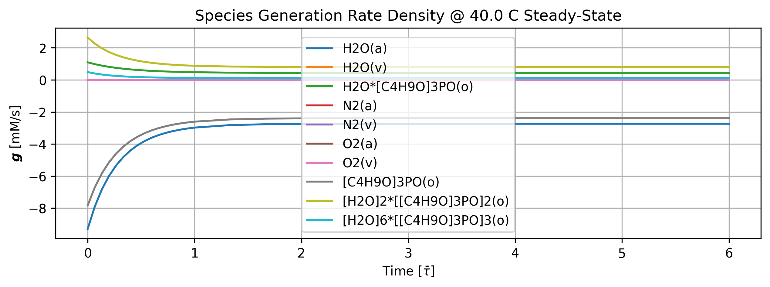
Figure 24: Species generation rate density history at steady-state.

tbl_count += 1
print(f'Table {tbl_count}: Species generation rate density history at steady-state.')
print('Time [min]        g [mM/s]')
import pandas as pd
col_names = [f'a{i}' for i in range(len(stg.rxn_mech.species_names))]
time_name = 't [min]'
df = (quant.value.apply(pd.Series).mul(1)
       .rename(index=lambda i: round(i/unit.min,2))
       .set_axis(col_names, axis=1).rename_axis(time_name)
       .round(4))
print(df.iloc[n_startup:].to_string(max_rows=20, min_rows=20))

Table 22: Species generation rate density history at steady-state.
Time [min]        g [mM/s]
             a0      a1      a2      a3      a4      a5      a6      a7      a8      a9
t [min]                                                                                
1.15    -2.8201  0.0014  0.4504  0.0027 -0.0027  0.0014 -0.0014 -2.4670  0.8324  0.1172
1.43    -2.7667  0.0014  0.4385  0.0027 -0.0027  0.0014 -0.0014 -2.4178  0.8159  0.1158
1.72    -2.7488  0.0014  0.4331  0.0027 -0.0027  0.0014 -0.0014 -2.4003  0.8100  0.1157
2.01    -2.7429  0.0014  0.4306  0.0027 -0.0027  0.0014 -0.0014 -2.3940  0.8080  0.1158
2.29    -2.7411  0.0014  0.4294  0.0027 -0.0027  0.0014 -0.0014 -2.3918  0.8072  0.1160
2.58    -2.7406  0.0014  0.4288  0.0027 -0.0027  0.0014 -0.0014 -2.3910  0.8070  0.1161
2.87    -2.7405  0.0014  0.4285  0.0027 -0.0027  0.0014 -0.0014 -2.3907  0.8069  0.1161
3.15    -2.7405  0.0014  0.4284  0.0027 -0.0027  0.0014 -0.0014 -2.3906  0.8069  0.1162
3.44    -2.7406  0.0014  0.4283  0.0027 -0.0027  0.0014 -0.0014 -2.3906  0.8069  0.1162
3.73    -2.7406  0.0014  0.4283  0.0027 -0.0027  0.0014 -0.0014 -2.3906  0.8069  0.1162
4.01    -2.7406  0.0014  0.4282  0.0027 -0.0027  0.0014 -0.0014 -2.3906  0.8069  0.1162
4.30    -2.7406  0.0014  0.4282  0.0027 -0.0027  0.0014 -0.0014 -2.3906  0.8069  0.1162
4.59    -2.7406  0.0014  0.4282  0.0027 -0.0027  0.0014 -0.0014 -2.3906  0.8069  0.1162
4.87    -2.7406  0.0014  0.4282  0.0027 -0.0027  0.0014 -0.0014 -2.3906  0.8069  0.1162
5.16    -2.7406  0.0014  0.4282  0.0027 -0.0027  0.0014 -0.0014 -2.3906  0.8069  0.1162

'''Produced species generation rate density'''
import matplotlib.pyplot as plt

ids, quant_produced = stg.g_vec_history(produced=True) # mole/m^3-s

quant_produced.plot(title='Produced Species Generation Rate Density @ %2.1f C Steady-State'%unit.convert_temperature(stg_temperature,
           'K','C'), x_scaling=1/stg.flow_residence_time_avg, x_label=r'Time [$\bar{\tau}$]', y_label=quant.latex_name+
           ' ['+quant_produced.unit+']', legend=list(np.array(stg.rxn_mech.species_names)[ids]), show=True, figsize=[10,3], error_data=False)

fig_count += 1
print(f'Figure {fig_count}: Produced species generation rate density history at steady-state.')

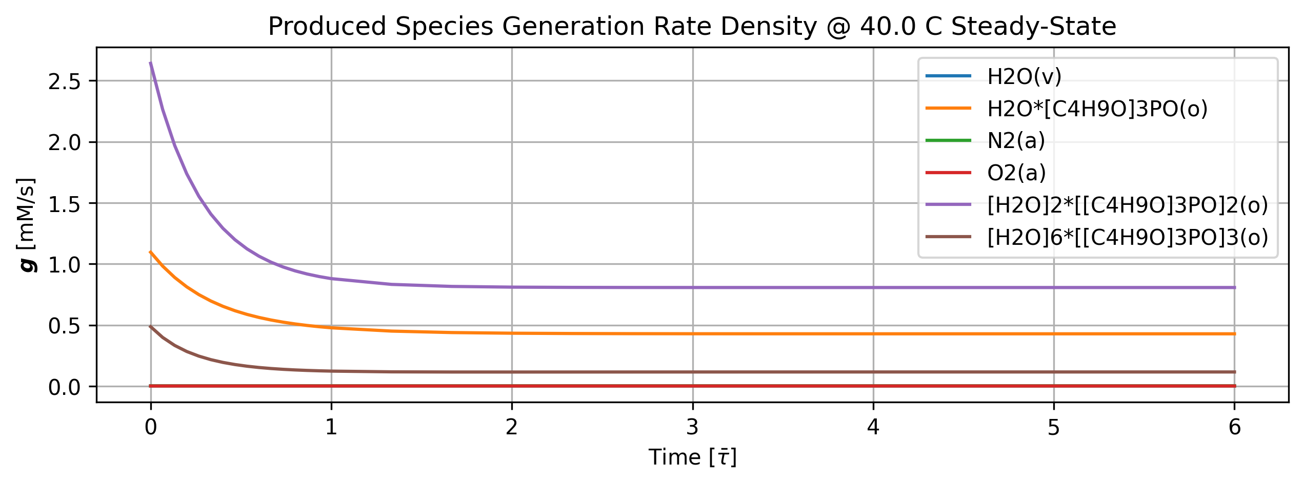
Figure 25: Produced species generation rate density history at steady-state.

if cortix_ai:
    issues = ('+ Title your reponse as: Overview of Species Generation Rates Density at Steady-State.\n'
              '+ Do not explain the start-up process; cover the steady-state only.'
)
    cortix_ai.explain(quant=quant, issues=issues, markdown_header_level='<h4>', markdown_display=markdown_display, print_prompt=False, save_supporting_info=db_save)

Cortix AI assistant: working on explanation...

Overview of Species Generation Rates Density at Steady-State.

Steady-state values (mM/s)

• H₂O(a): -2.74061 mM/s (net consumption)

• H₂O(v): 0.00135593 mM/s (net production)

• H₂O·[C₄H₉O]₃PO(o): 0.428226 mM/s (net production)

• N₂(a): 0.00269596 mM/s (net production)

• N₂(v): -0.00269596 mM/s (net consumption)

• O₂(a): 0.00142770 mM/s (net production)

• O₂(v): -0.00142770 mM/s (net consumption)

• [C₄H₉O]₃PO(o): -2.39059 mM/s (net consumption)

• [H₂O]₂·[[C₄H₉O]₃PO]₂(o): 0.806856 mM/s (net production)

• [H₂O]₆·[[C₄H₉O]₃PO]₃(o): 0.116219 mM/s (net production)

Key steady-state observations

• Dominant fluxes: the largest-magnitude rates are consumption of H₂O(a) (≈ -2.74 mM/s) and [C₄H₉O]₃PO(o) (≈ -2.39 mM/s), and production of the hydrated/adduct complexes (especially [H₂O]₂·[[C₄H₉O]₃PO]₂(o) at ≈ 0.8069 mM/s).

• Phase-exchange pairs (N₂ and O₂): N₂(a) and N₂(v) are equal in magnitude and opposite in sign (±0.00269596 mM/s); O₂(a) and O₂(v) are likewise equal/opposite (±0.00142770 mM/s). This indicates steady-state phase transfer between adsorbed and vapor forms with negligible net creation/destruction beyond exchange.

• Relative significance: water- and organophosphate-related species carry the bulk of the generation/consumption (orders of magnitude larger than the dilute gas-phase rates listed).

• Numerical steadiness: values are essentially constant across the final time entries (t ≥ ~100 s in the table), so the listed numbers represent the steady-state generation-rate density in mM/s.

AI Parameters:
+ LLM model (OpenAI) = gpt-5-mini
+ LLM cleverness     = 1.0
+ Total # of tokens  = 5896

1.6.7. Mass Balance Residual

This is actually the total mass generation rate density (mixing volume) residual; a small number in view of total mass conservation.

'''Mass balance residuals'''
import matplotlib.pyplot as plt

quant = stg.mass_balance_residual_history()

quant.plot(title='Total Mass Generation Rate Density @ %2.1f C Steady-State'%unit.convert_temperature(stg_temperature,
           'K','C'), x_scaling=1/stg.flow_residence_time_avg, x_label=r'Time [$\bar{\tau}$]', y_label=quant.latex_name+
           ' ['+quant.unit+']', markers_only=True, legend=['Residual'], show=True, figsize=[10,3])

fig_count += 1
print(f'Figure {fig_count}: Total mass generation rate density residual history at steady-state.')

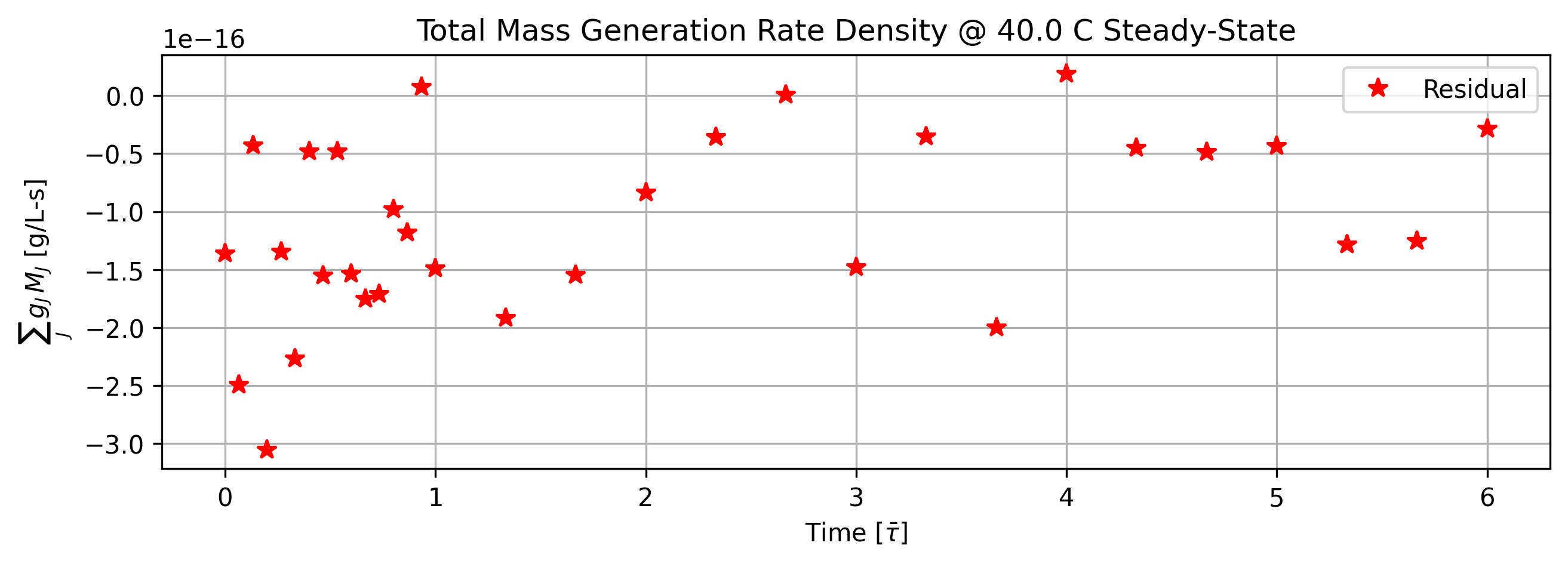
Figure 26: Total mass generation rate density residual history at steady-state.

if cortix_ai:
    issues = ('+ Title your reponse as: Total Mass Generation Rate Density Residual at Steady-State.\n'
             '+ Do not explain the start-up process; cover the steady-state only.'
    )
    cortix_ai.explain(quant=quant, issues=issues, markdown_header_level='<h4>', markdown_display=markdown_display, print_prompt=False, save_supporting_info=db_save)

Cortix AI assistant: working on explanation...

Total Mass Generation Rate Density Residual at Steady-State.

Data selection

• Steady-state interval inspected: t = 103.208 s through 309.624 s (rows with times 103.208, 154.812, 206.416, 258.02, 309.624); N = 5 samples.

Numeric summary (steady-state samples)

• Time column:

  • min = 103.208 s, max = 309.624 s, mean = 206.416 s, sampling step ≈ 51.604 s (uniform spacing in this subset).

• Total Mass Generation Rate Density [g/L-s] (steady-state values):

  • values = [−8.39579e-17, −1.47926e-16, 1.88719e-17, −4.34833e-17, −2.84061e-17]

  • mean = −5.70e-17 g/L-s

  • median = −4.35e-17 g/L-s

  • standard deviation ≈ 5.61e-17 g/L-s

  • RMS ≈ 8.00e-17 g/L-s

  • minimum (most negative) = −1.47926e-16 g/L-s

  • maximum (most positive) = 1.88719e-17 g/L-s

  • maximum absolute residual = 1.47926e-16 g/L-s

• Linear trend (least-squares slope of residual vs time over the steady-state interval):

  • slope ≈ 4.2e-19 g·L⁻¹·s⁻2 (i.e., g/L-s change per second), effectively zero within numerical noise.

Interpretation

• The mass-generation residuals during the steady-state interval are centered near zero (mean ≈ −5.7×10⁻¹⁷ g/L-s) with scatter on the order of 10⁻¹⁷–10⁻¹⁶ g/L-s.

• No significant systematic drift is visible (slope ≈ 4.2×10⁻¹⁹ g/L-s per s); the largest discrepancy is ~1.48×10⁻¹⁶ g/L-s.

• Conclusion: mass balance in the mixing volume is satisfied to within O(10⁻¹⁶) g/L-s during the inspected steady-state interval, consistent with numerical round-off / solver residual levels.

AI Parameters:
+ LLM model (OpenAI) = gpt-5-mini
+ LLM cleverness     = 1.0
+ Total # of tokens  = 7492

'''Time for 1 gram imbalance in variable volumes'''

time = ( (1*unit.gram/(10000*unit.gallon)) / abs(quant.value.mean()) ) / unit.year
print('Time for imbalance of 1 gram in 10000 gallons: %1.1f [years]'%time)

time = ( (1*unit.gram/(1e6*unit.gallon)) / abs(quant.value.mean()) ) / unit.year
print('Time for imbalance of 1 gram in 1e6 gallons: %1.1f [years]'%time)

Time for imbalance of 1 gram in 10000 gallons: 7517.2 [years]
Time for imbalance of 1 gram in 1e6 gallons: 75.2 [years]

1.7. Shut-down Simulation

From steady-state, shutdown in two flow residence times.

end_time += 3 * stg.flow_residence_time_avg
time_step = 3 * stg.flow_residence_time_avg / 20
show_time = (True, 10*time_step)

stg.time_step = time_step
stg.initial_time = stg.end_time
stg.end_time = end_time
stg.show_time = show_time

'''Abrupt turn-off of TBP concentration in the organic phase in the inflow'''
tbp_mass_cc_org = 0.0
stg.inflow_organic_phase.set_value(tbp_org_name, tbp_mass_cc_org)

'''Run system in parallel'''
stg.monitor_mass_flowrates = False
stg.monitor_mass_conservation_residual = False
system.run()
system.close() # Shutdown Cortix

[31384] 2025-12-02 16:01:22,348 - cortix - INFO - Launching Module <solvex.stage.Stage object at 0x7f853d903610>
[2417] 2025-12-02 16:01:23,618 - cortix - INFO - Stg-1::run():time[m]=5.2
[2417] 2025-12-02 16:01:23,976 - cortix - INFO - Stg-1::run():time[m]=6.5
Total mass rate density (mixture volume) residual [g/L-s]= 6.64074e-19
total mass inflow rate [g/min]   = 4.961e+02
total mass outflow rate [g/min]  =  5.045e+02
	 net total mass flow rate [g/min] = 8.396e+00
[2417] 2025-12-02 16:01:24,316 - cortix - INFO - Stg-1::run():time[m]=7.7 (et[s]=0.7)
[31384] 2025-12-02 16:01:24,479 - cortix - INFO - run()::Elapsed wall clock time [s]: 1272.14
[31384] 2025-12-02 16:01:24,480 - cortix - INFO - Closed Cortix object.
_____________________________________________________________________________
                           T E R M I N A T I N G                             
_____________________________________________________________________________
      ...                                        s       .     (TAAG Fraktur)
   xH88"`~ .x8X                                 :8      @88>
 :8888   .f"8888Hf        u.      .u    .      .88      %8P      uL   ..
:8888>  X8L  ^""`   ...ue888b   .d88B :@8c    :888ooo    .     .@88b  @88R
X8888  X888h        888R Y888r ="8888f8888r -*8888888  .@88u  ""Y888k/"*P
88888  !88888.      888R I888>   4888>"88"    8888    888E`    Y888L
88888   %88888      888R I888>   4888> "      8888      888E      8888
88888 `> `8888>     888R I888>   4888>        8888      888E      `888N
`8888L %  ?888   ! u8888cJ888   .d888L .+    .8888Lu=   888E   .u./"888&
 `8888  `-*""   /   "*888*P"    ^"8888*"     ^%888*     888&  d888" Y888*"
   "888.      :"      "Y"          "Y"         "Y"      R888" ` "Y   Y"
     `""***~"`                                           ""
                             https://cortix.org                              
_____________________________________________________________________________
[31384] 2025-12-02 16:01:24,481 - cortix - INFO - close()::Elapsed wall clock time [s]: 1272.15

'''Recover stage'''
stg = system_net.modules[0]

1.7.1. Organic Phase Results

'''Plot organic phase'''
# TODO: time axis normalized by phase flow residence time.
stg.organic_phase.plot(title='Organic Phase Shut-Down', legend='Organic Phase', nrows=2,ncols=3, show=True, figsize=[12,6])

fig_count += 1
print(f'Figure {fig_count}: Organic phase species history dashboard at shut-down.')

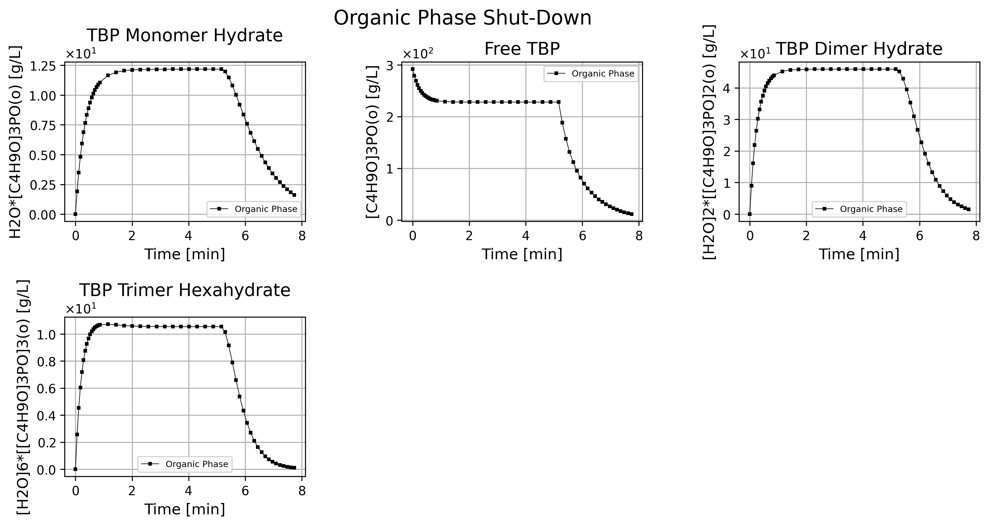
Figure 27: Organic phase species history dashboard at shut-down.

if cortix_ai:
    issues = ('+ Title your reponse as: Overview of the Organic Phase Data at Shut-Down.\n'
              f'+ Cover only the period after {round(stg.initial_time,2)} seconds when the concentration of TBP in the inflow is set to zero.'
    )
    cortix_ai.explain(phase=stg.organic_phase, issues=issues, markdown_header_level='<h4>', markdown_display=markdown_display, print_prompt=False, save_supporting_info=db_save)

Cortix AI assistant: working on explanation...

Overview of the Organic Phase Data at Shut-Down.

Scope

Data rows with time ≥ 309.624 s only (shut-down of TBP inflow at 309.624 s). All concentrations are in g/L; species notation used below follows the table but with corrected chemical formatting (H₂O·[C₄H₉O]₃PO(o), [C₄H₉O]₃PO(o), [H₂O]₂·[[C₄H₉O]₃PO]₂(o), [H₂O]₆·[[C₄H₉O]₃PO]₃(o)).

Key observations

• Immediately after shut-down (309.624 s → 317.365 s) TBP ([C₄H₉O]₃PO) shows a large drop from 228.085 to 188.653 g/L (≈ −39.43 g/L, −17.3%) within 7.741 s; the hydrate complexes show much smaller absolute changes in that same interval.

• Over the full post-shutdown interval analyzed (309.624 → 464.436 s, Δt = 154.812 s) all four measured organic-phase concentrations fall substantially.

• TBP remains the dominant component by mass at every sampled time after shut-down, even as absolute TBP concentration declines strongly.

• The hydrated complexes decline as well; the dihydrate complex has the largest absolute concentration decline after TBP, while the trimer hydrate declines to nearly zero by 464.436 s.

Quantitative changes (309.624 s → 464.436 s)

• H₂O·[C₄H₉O]₃PO(o): 12.1757 → 1.60434 g/L; absolute change −10.57136 g/L; fractional decrease ≈ 86.9%; mean rate ≈ −0.0683 g·L⁻¹·s⁻¹.

• [C₄H₉O]₃PO(o) (TBP): 228.085 → 11.4963 g/L; absolute change −216.5887 g/L; fractional decrease ≈ 95.0%; mean rate ≈ −1.399 g·L⁻¹·s⁻¹.

• [H₂O]₂·[[C₄H₉O]₃PO]₂(o): 45.8827 → 1.53375 g/L; absolute change −44.34895 g/L; fractional decrease ≈ 96.7%; mean rate ≈ −0.287 g·L⁻¹·s⁻¹.

• [H₂O]₆·[[C₄H₉O]₃PO]₃(o): 10.5415 → 0.102006 g/L; absolute change −10.43949 g/L; fractional decrease ≈ 99.0%; mean rate ≈ −0.0674 g·L⁻¹·s⁻¹.

• Total organic-phase concentration (sum of the four species): 296.685 → 14.7364 g/L; absolute change −281.949 g/L; fractional decrease ≈ 95.0%.

Temporal pattern and notable transient

• Two-phase behavior is evident: an initial abrupt drop in TBP immediately after 309.624 s (largest short-term change), followed by a smoother, roughly monotonic decline of all species over the remaining time points.

• The hydrate complexes decline more slowly in the initial few seconds compared with TBP, but over the full interval they fall almost as far (dihydrate shows the largest absolute loss among hydrates).

• By the end of the analyzed interval (464.436 s) monohydrate and dihydrate concentrations remain nonzero but small; the trimer hydrate is effectively depleted (<0.11 g/L).

Composition and relative shares

• At 309.624 s the composition by mass fraction was approx.: TBP 76.9%, dihydrate 15.5%, monohydrate 4.1%, trimer hydrate 3.6%.

• At 464.436 s the mass fractions are approx.: TBP 78.0%, monohydrate 10.9%, dihydrate 10.4%, trimer hydrate 0.7% — TBP retains the largest share despite large absolute loss.

• The data show the bulk of organic mass is removed/depleted after shut-down, with TBP and the dihydrate accounting for most of the absolute mass loss.

Concise conclusion

• After inflow of TBP is set to zero at 309.624 s, the organic-phase concentrations decline rapidly: TBP and the dihydrate exhibit the largest absolute decreases and dominate the total mass loss, while the monohydrate and trimer hydrate also fall to low values (trimer near zero) over ~155 s.

AI Parameters:
+ LLM model (OpenAI) = gpt-5-mini
+ LLM cleverness     = 1.0
+ Total # of tokens  = 8294

'''Compute molar concentration of TBP species'''
import numpy as np

tbp_mass_cc_org_history = stg.organic_phase.get_column(tbp_org_name)
tbp_molar_cc_org_history = np.array(tbp_mass_cc_org_history)/tbp_org.molar_mass

tbp_monomer_mass_cc_org_history = stg.organic_phase.get_column(tbp_monomer_org_name)
tbp_monomer_molar_cc_org_history = np.array(tbp_monomer_mass_cc_org_history)/tbp_monomer_org.molar_mass

tbp_dimer_mass_cc_org_history = stg.organic_phase.get_column(tbp_dimer_org_name)
tbp_dimer_molar_cc_org_history = np.array(tbp_dimer_mass_cc_org_history)/tbp_dimer_org.molar_mass

tbp_trimer_hexahydrate_mass_cc_org_history = stg.organic_phase.get_column(tbp_trimer_hexahydrate_org_name)
tbp_trimer_hexahydrate_molar_cc_org_history = np.array(tbp_trimer_hexahydrate_mass_cc_org_history)/tbp_trimer_hexahydrate_org.molar_mass

time_stamps = np.array(stg.organic_phase.time_stamps)

tbl_count += 1
print(f'Table {tbl_count}: Molarity history of TBP in the organic phase at shut-down.')
print('Time [min] | Free TBP [M] | TBP Monomer [M] | TBP Dimer [M] | TBP Trimer Hexahydrate [M] | balance |')
np.set_printoptions(precision=3, suppress=True, linewidth=100)
for t,a,b,c,d in zip(time_stamps[n_startup::5]/unit.min, 
                 tbp_molar_cc_org_history[n_startup::5]/unit.molar, 
                 tbp_monomer_molar_cc_org_history[n_startup::5]/unit.molar,
                 tbp_dimer_molar_cc_org_history[n_startup::5]/unit.molar,
                 tbp_trimer_hexahydrate_molar_cc_org_history[n_startup::5]/unit.molar):
    balance = a+b+2*c+3*d - tbp_mass_cc_org/tbp_org.molar_mass/unit.molar
    print('  %1.2e      %1.3f         %1.3e        %1.3e               %1.3e          %+1.3e'%(t, a, b, c, d, balance))

Table 23: Molarity history of TBP in the organic phase at shut-down.
Time [min] | Free TBP [M] | TBP Monomer [M] | TBP Dimer [M] | TBP Trimer Hexahydrate [M] | balance |
  1.15e+00      0.860         4.097e-02        7.950e-02               1.182e-02          +1.096e+00
  2.58e+00      0.856         4.277e-02        8.068e-02               1.164e-02          +1.096e+00
  4.01e+00      0.856         4.282e-02        8.069e-02               1.162e-02          +1.096e+00
  5.29e+00      0.708         4.215e-02        7.942e-02               1.118e-02          +9.429e-01
  5.93e+00      0.308         2.947e-02        4.699e-02               4.766e-03          +4.454e-01
  6.58e+00      0.151         1.720e-02        1.919e-02               1.379e-03          +2.104e-01
  7.22e+00      0.076         9.413e-03        6.705e-03               3.516e-04          +9.938e-02

'''Volume fraction of TBP at shut-down'''
tbl_count += 1
print(f'Table {tbl_count}: Volume fractions of free and total TBP in the organic phase at shut-down.')
print('Time [min] | Free TBP vol frac [%] | Total TBP vol frac [%] |')
np.set_printoptions(precision=3, suppress=True, linewidth=100)
total_tbp_molar_cc_org_history = tbp_molar_cc_org_history + tbp_monomer_molar_cc_org_history + \
                                 2*tbp_dimer_molar_cc_org_history + 3*tbp_trimer_hexahydrate_molar_cc_org_history
total_tbp_mass_cc_org_history = total_tbp_molar_cc_org_history * tbp_org.molar_mass
for t,a,b in zip(time_stamps[::5]/unit.min, 
               np.array(tbp_mass_cc_org_history[::5])/rho_tbp*100, total_tbp_mass_cc_org_history[::5]/rho_tbp*100):
    print('  %1.2e         %1.3f                  %1.3f'%(t, a, b))

Table 24: Volume fractions of free and total TBP in the organic phase at shut-down.
Time [min] | Free TBP vol frac [%] | Total TBP vol frac [%] |
  0.00e+00         30.000                  30.000
  2.87e-01         25.701                  30.000
  5.73e-01         24.244                  30.000
  8.60e-01         23.734                  30.000
  2.29e+00         23.455                  30.000
  3.73e+00         23.453                  30.000
  5.16e+00         23.453                  30.000
  5.81e+00         9.815                  14.171
  6.45e+00         4.742                  6.694
  7.10e+00         2.375                  3.162
  7.74e+00         1.182                  1.494

'''Total water extracted'''
water_molar_cc_org_history = tbp_monomer_molar_cc_org_history \
                           + 2*tbp_dimer_molar_cc_org_history \
                           + 6*tbp_trimer_hexahydrate_molar_cc_org_history

water_mass_cc_org_history = water_molar_cc_org_history * h2o_aqu.molar_mass

tbl_count += 1
print(f'Table {tbl_count}: Mass concentration and molarity history of water in the organic phase at shut-down.')
print('Time [s] |   [M]   |  [g/L]  |')
np.set_printoptions(precision=3, suppress=True, linewidth=100)
for a,b,c in zip(time_stamps[n_startup::5], water_molar_cc_org_history[n_startup::5]/unit.molar, water_mass_cc_org_history[n_startup::5]):
    print('%1.2e  %1.3e %1.3e'%(a, b, c))

Table 25: Mass concentration and molarity history of water in the organic phase at shut-down.
Time [s] |   [M]   |  [g/L]  |
6.88e+01  2.709e-01 4.880e+00
1.55e+02  2.739e-01 4.935e+00
2.41e+02  2.739e-01 4.935e+00
3.17e+02  2.681e-01 4.829e+00
3.56e+02  1.520e-01 2.739e+00
3.95e+02  6.385e-02 1.150e+00
4.33e+02  2.493e-02 4.492e-01

'''Organic phase mass density'''
import matplotlib.pyplot as plt

quant = stg.mass_density_history('organic')

quant.plot(title='Organic Phase Mass Density @ %2.1f C Shut-Down'%unit.convert_temperature(stg_temperature,
           'K','C'), x_scaling=1/stg.flow_residence_time_avg, x_label=r'Time [$\bar{\tau}$]', y_label=quant.latex_name+r'$-\rho_\text{diluent}$'
           ' ['+quant.unit+']', show=True, figsize=[10,3], error_data=False)

fig_count += 1
print(f'Figure {fig_count}: Organic phase mass density history at shut-down.')

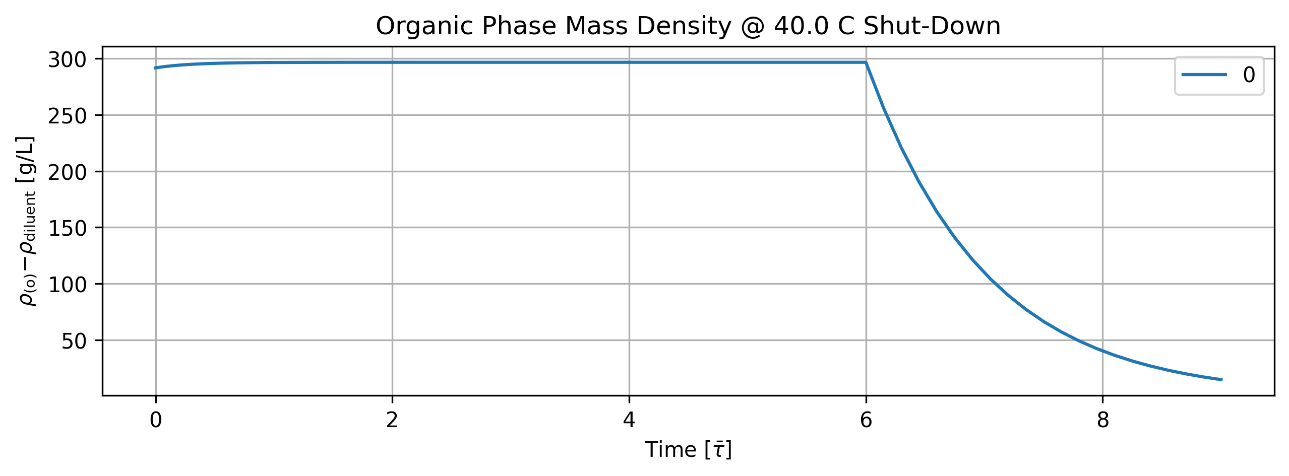
Figure 28: Organic phase mass density history at shut-down.

tbl_count += 1
print(f'Table {tbl_count}: Organic phase mass density history at shut-down.')
print('Time [s]  Organic Phase Mass Density [g/L]')
print(quant.value[::5].apply(lambda x: round(x,2)))

Table 26: Organic phase mass density history at shut-down.
Time [s]  Organic Phase Mass Density [g/L]
0.000000      291.75
17.201342     295.06
34.402683     296.14
51.604025     296.51
137.610734    296.69
223.617442    296.68
309.624151    296.68
348.327170    141.00
387.030188     66.48
425.733207     31.29
464.436226     14.74
Name: Organic Phase Mass Density [g/L]; Time History in [s], dtype: float64

1.7.2. Aqueous Phase Results

'''Plot aqueous phase'''
# TODO: time axis normalized by phase flow residence time.
stg.aqueous_phase.plot(title='Aqueous Phase Shut-Down', legend='Aqueous Phase', nrows=2,ncols=3, show=True, figsize=[12,6])

fig_count += 1
print(f'Figure {fig_count}: Aqueous phase species history dashboard at shut-down.')

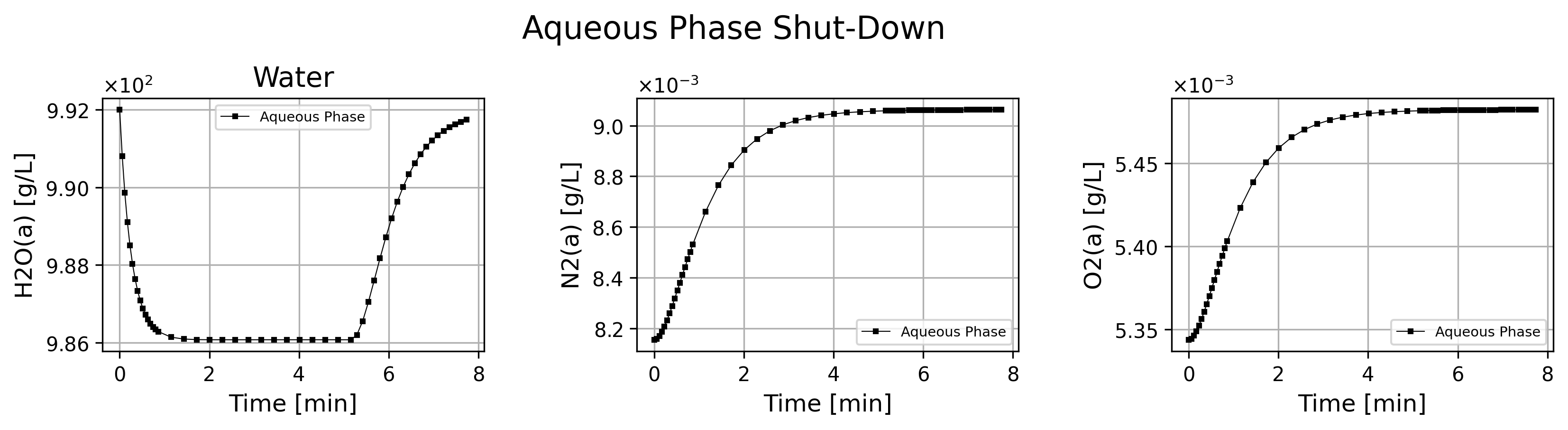
Figure 29: Aqueous phase species history dashboard at shut-down.

if cortix_ai:
    issues = ('+ Title your reponse as: Overview of the Aqueous Phase Data at Shut-Down.\n'
              f'+ Cover only the period after {round(stg.initial_time,2)} seconds when the concentration of TBP in the inflow is set to zero.'
    )
    cortix_ai.explain(phase=stg.aqueous_phase, issues=issues, markdown_header_level='<h4>', markdown_display=markdown_display, save_supporting_info=db_save)

Cortix AI assistant: working on explanation...

Overview of the Aqueous Phase Data at Shut-Down.

Period considered

• Analysis restricted to measurements at and after 309.624 s (rows with time ≥ 309.624 s); this is the period after the inflow TBP concentration is set to zero.

Key numeric changes (309.624 s -> 464.436 s)

• H₂O(a): 986.075 g/L -> 991.744 g/L; absolute change +5.669 g/L; relative change +0.575%; mean rate ≈ 0.0366 g·L⁻¹·s⁻¹.

• N₂(a): 0.00905861 g/L -> 0.00906259 g/L; absolute change +3.98×10⁻⁶ g/L; relative change ≈ +0.0439%; mean rate ≈ 2.57×10⁻⁸ g·L⁻¹·s⁻¹.

• O₂(a): 0.00548158 g/L -> 0.00548215 g/L; absolute change +5.7×10⁻⁷ g/L; relative change ≈ +0.0104%; mean rate ≈ 3.68×10⁻⁹ g·L⁻¹·s⁻¹.

Temporal patterns within the period

• H₂O(a) shows a clear upward trend beginning immediately after 309.624 s: a relatively faster rise between ~309.6 s and ~340.6 s, then a slower approach toward ~991.7 g/L by 464.4 s (behavior consistent with a transient response toward a new equilibrium).

• N₂(a) and O₂(a) both increase only very slightly and almost linearly over this interval; their absolute and relative changes are negligible compared with the change in H₂O(a).

Comparative significance

• The H₂O(a) change dominates the aqueous-phase mass balance after shut-down: its absolute increase (~5.67 g/L) is several orders of magnitude larger than the changes in dissolved N₂(a) and O₂(a).

• Changes in dissolved gases (N₂ and O₂) are sub-ppm in magnitude relative to H₂O and are unlikely to be significant for bulk mass unless the system is sensitive to trace gas concentrations.

Concise interpretation

• After the inflow TBP is set to zero, the aqueous phase exhibits a pronounced increase in H₂O(a) concentration that moves toward a new steady value over ~150 s, while dissolved N₂(a) and O₂(a) remain effectively constant (very small increases). This indicates a dominant water concentration adjustment in the post-shutdown transient.

AI Parameters:
+ LLM model (OpenAI) = gpt-5-mini
+ LLM cleverness     = 1.0
+ Total # of tokens  = 6456

'''Aqueous phase mass density'''
import matplotlib.pyplot as plt

quant = stg.mass_density_history('aqueous')

quant.plot(title='Aqueous Phase Mass Density @ %2.1f C Shut-Down'%unit.convert_temperature(stg_temperature,
           'K','C'), x_scaling=1/stg.flow_residence_time_avg, x_label=r'Time [$\bar{\tau}$]', y_label=quant.latex_name+
           ' ['+quant.unit+']', show=True, figsize=[10,3], error_data=False)

fig_count += 1
print(f'Figure {fig_count}: Aqueous phase mass density history at shut-down.')

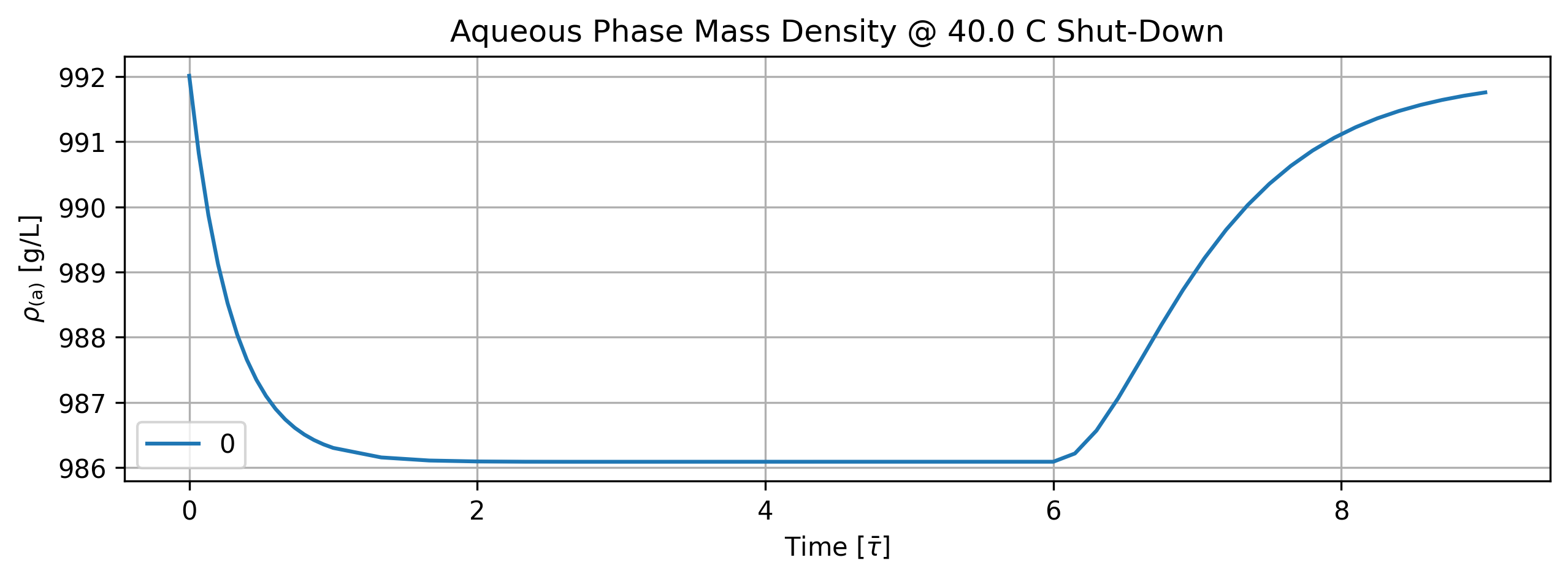
Figure 30: Aqueous phase mass density history at shut-down.

tbl_count += 1
print(f'Table {tbl_count}: Aqueous phase mass density history at shut-down.')
print('Time [s]  Aqueous Phase Mass Density [g/L]')
print(quant.value[::5].apply(lambda x: round(x,2)))

Table 27: Aqueous phase mass density history at shut-down.
Time [s]  Aqueous Phase Mass Density [g/L]
0.000000      992.01
17.201342     988.04
34.402683     986.74
51.604025     986.30
137.610734    986.09
223.617442    986.09
309.624151    986.09
348.327170    988.19
387.030188    990.35
425.733207    991.36
464.436226    991.76
Name: Aqueous Phase Mass Density [g/L]; Time History in [s], dtype: float64

1.7.3. Vapor Phase Results

'''Plot vapor phase'''
# TODO: time axis normalized by phase flow residence time.
stg.vapor_phase.plot(title='Vapor Phase Shut-Down', legend='Vapor Phase', nrows=2,ncols=3, show=True, figsize=[12,6])

fig_count += 1
print(f'Figure {fig_count}: Vapor phase species history dashboard at shut-down.')

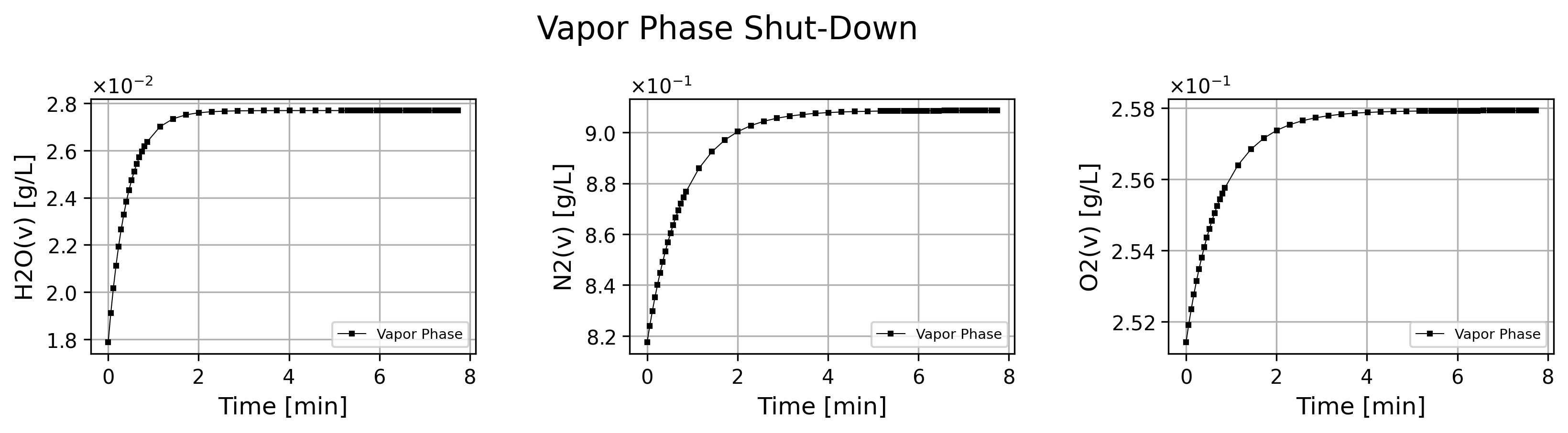
Figure 31: Vapor phase species history dashboard at shut-down.

if cortix_ai:
    issues = ('+ Title your reponse as: Overview of the Vapor Phase Data at Shut-Down.\n'
              f'+ Cover only the period after {round(stg.initial_time,2)} seconds when the concentration of TBP in the inflow is set to zero.'
    )
    cortix_ai.explain(phase=stg.vapor_phase, issues=issues, markdown_header_level='<h4>', markdown_display=markdown_display, save_supporting_info=db_save)

Cortix AI assistant: working on explanation...

Overview of the Vapor Phase Data at Shut-Down.

Data subset and time window

• Data shown: all rows with time ≥ 309.624 s (start at 309.624 s and end at 464.436 s).

• Number of samples in this window: 21 samples spanning Δt = 464.436 − 309.624 = 154.812 s.

Column-by-column numerical summary (post 309.624 s)

• time [s]

  • Range: 309.624 → 464.436 s; evenly sampled points within that interval (21 entries).

• concentration of H₂O(v) [g/L]

  • Values: essentially constant at ≈ 0.0276972 g/L (visible digits: 0.0276971–0.0276972).

  • Change over window: ≈ +1×10⁻⁷ g/L (negligible).

• concentration of N₂(v) [g/L]

  • Values: increase from 0.908398 → 0.908598 g/L.

  • Absolute change: +0.000200 g/L.

  • Relative change: ≈ +0.022% of the initial value.

• concentration of O₂(v) [g/L]

  • Values: increase from 0.257921 → 0.257934 g/L.

  • Absolute change: +0.000013 g/L.

  • Relative change: ≈ +0.005% of the initial value.

Trends and approximate rates

• H₂O(v): effectively steady — slope ≈ 6.5×10⁻¹⁰ g·L⁻¹·s⁻¹ (practically zero for the sampling resolution).

• N₂(v): small positive linear trend — slope ≈ 1.29×10⁻⁶ g·L⁻¹·s⁻¹.

• O₂(v): very small positive trend — slope ≈ 8.4×10⁻⁸ g·L⁻¹·s⁻¹.

• All three species show either negligible change or very slow monotonic increases; no oscillations or abrupt shifts are present in this period.

Comparison and interpretation of behavior

• Magnitude: N₂ is dominant (~0.9086 g/L), O₂ is intermediate (~0.25793 g/L), H₂O is minor (~0.027697 g/L).

• Stability: H₂O exhibits the greatest fractional stability (practically invariant), while N₂ shows the largest absolute and relative incremental change over the period (but still very small: ~0.02%).

• Timescale: over ~155 s after TBP inflow set to zero, the vapor composition is effectively at steady state within the resolution of the recorded values; small residual rises in N₂ and O₂ are observed but are minute.

Concise conclusion

• After 309.624 s (TBP inflow = 0), the vapor-phase concentrations remain essentially steady for H₂O(v), N₂(v), and O₂(v). The only measurable changes are tiny, monotonic increases in N₂ and O₂ (order 10⁻⁴–10⁻⁵), while H₂O remains fixed to within 10⁻⁷ g/L. Overall the vapor composition is stable on the sampled timescale.

AI Parameters:
+ LLM model (OpenAI) = gpt-5-mini
+ LLM cleverness     = 1.0
+ Total # of tokens  = 5886

'''Vapor phase mass density'''
import matplotlib.pyplot as plt

quant = stg.mass_density_history('vapor')

quant.plot(title='Vapor Phase Mass Density @ %2.1f C Shut-Down'%unit.convert_temperature(stg_temperature,
           'K','C'), x_scaling=1/stg.flow_residence_time_avg, x_label=r'Time [$\bar{\tau}$]', y_label=quant.latex_name+
           ' ['+quant.unit+']', show=True, figsize=[10,3], error_data=False)

fig_count += 1
print(f'Figure {fig_count}: Vapor phase mass density history at shut-down.')

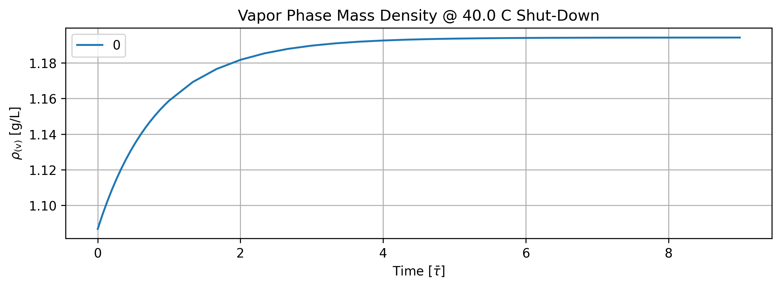
Figure 32: Vapor phase mass density history at shut-down.

tbl_count += 1
print(f'Table {tbl_count}: Vapor phase mass density history at shut-down.')
print('Time [s]  Vapor Phase Mass Density [g/L]')
print(quant.value[::5].apply(lambda x: round(x,2)))

Table 28: Vapor phase mass density history at shut-down.
Time [s]  Vapor Phase Mass Density [g/L]
0.000000      1.09
17.201342     1.12
34.402683     1.14
51.604025     1.16
137.610734    1.19
223.617442    1.19
309.624151    1.19
348.327170    1.19
387.030188    1.19
425.733207    1.19
464.436226    1.19
Name: Vapor Phase Mass Density [g/L]; Time History in [s], dtype: float64

1.7.3.1. Relative Humidity

'''Compute relative humidity in the vapor phase'''
import matplotlib.pyplot as plt
from solvex import air_relative_humidity
from copy import deepcopy

h2o_vap_pd_series = deepcopy(stg.vapor_phase.df['H2O(v)'])
for idx, rho_h2o in enumerate(h2o_vap_pd_series):
    h2o_vap_pd_series.iloc[idx] = air_relative_humidity(stg_temperature, rho_h2o)
rh_pd_series = h2o_vap_pd_series
time_unit = stg.vapor_phase.time_unit
rh_pd_series.name = f'Relative Humidity History [{time_unit}]'
  
quant = Quantity(name=rh_pd_series.name, latex_name='RH', unit='%', info=f'Relative Humidity History (Vapor Phase) [{time_unit}]')
quant.value = h2o_vap_pd_series
quant.plot(title='Stage Rel. Humidity @ %2.1f C Shut-Down'%unit.convert_temperature(stg_temperature, 'K','C'),
           x_scaling=1/stg.flow_residence_time_avg, x_label=r'Time [$\bar{\tau}$]', y_label=quant.latex_name+' ['+quant.unit+']', show=True, 
           figsize=[10,3])

fig_count += 1
print(f'Figure {fig_count}: Stage relative humidity history at shut-down.')

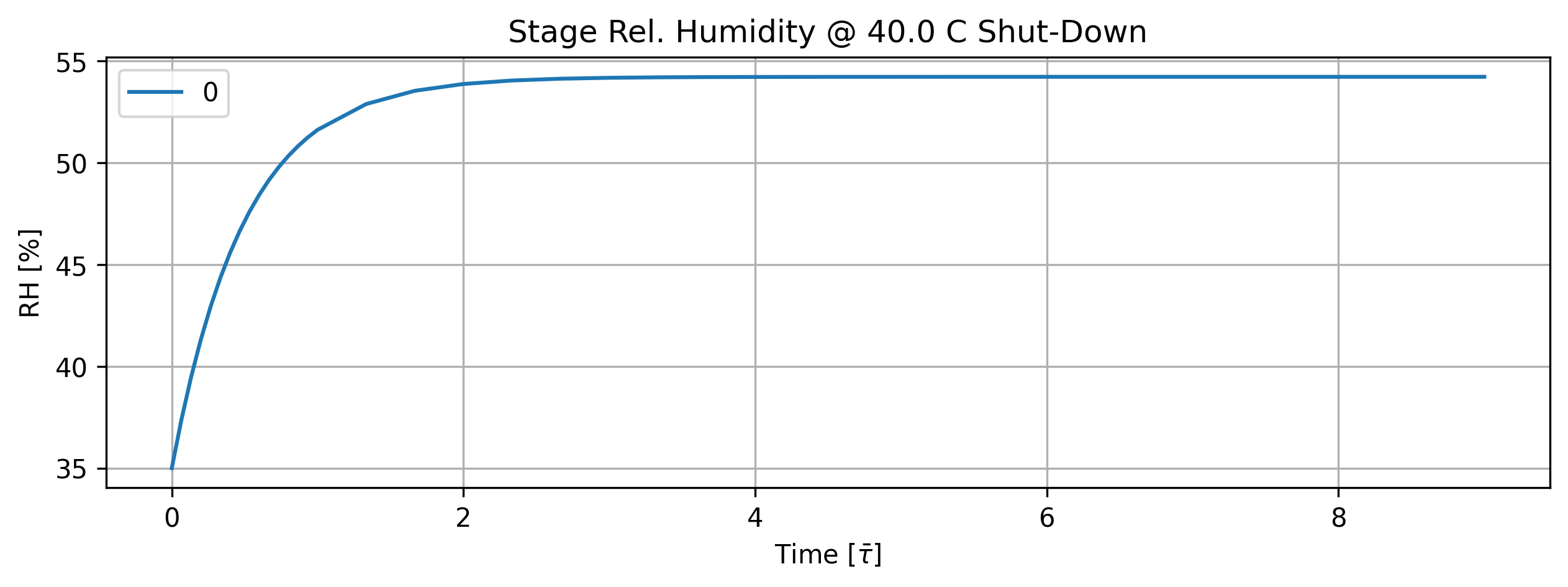
Figure 33: Stage relative humidity history at shut-down.

tbl_count += 1
print(f'Table {tbl_count}: Stage relative humidity history at shut-down.')
print('Time [s]  Rel. Humidity [%]')
print(quant.value.loc[n_startup::5].apply(lambda x: round(x,2)))

Table 29: Stage relative humidity history at shut-down.
Time [s]  Rel. Humidity [%]
17.201342     44.36
34.402683     49.16
51.604025     51.63
137.610734    54.14
223.617442    54.23
309.624151    54.23
348.327170    54.23
387.030188    54.23
425.733207    54.23
464.436226    54.23
Name: Relative Humidity History [s], dtype: float64

if cortix_ai:
    issues = ('+ Title your reponse as: Overview of the Relative Humidity Data at Shut-Down.\n'
              f'+ Cover only the period after {round(stg.initial_time,2)} seconds when the concentration of TBP in the inflow is set to zero.'
    )
    cortix_ai.explain(quant=quant, issues=issues, markdown_header_level='<h5>', markdown_display=markdown_display, print_prompt=False, save_supporting_info=db_save)

Cortix AI assistant: working on explanation...

Overview of the Relative Humidity Data at Shut-Down.

Data considered

• Period analysed: all rows with time >= 309.624 s (the moment TBP inflow concentration is set to zero).

• Data points (time [s] → Relative Humidity [%]):

  • 309.624 → 54.2303

  • 356.068 → 54.2304

  • 402.511 → 54.2304

  • 448.955 → 54.2304

Descriptive statistics (n = 4)

• Mean RH = 54.230375% (≈ 54.23038%).

• Minimum = 54.2303%; Maximum = 54.2304%; Range = 0.0001 percentage points.

• Standard deviation (population) ≈ 4.33e-5 %; sample standard deviation ≈ 5.00e-5 %.

• Observed values are identical to four decimal places except the first point (54.2303).

Temporal sampling

• Sampling intervals are nearly uniform:

  • 309.624 → 356.068: Δt = 46.444 s

  • 356.068 → 402.511: Δt = 46.443 s

  • 402.511 → 448.955: Δt = 46.444 s

• Small RH change between the first and second post-shutdown samples: ΔRH = +0.0001 over 46.444 s → ≈ 2.15e-6 %/s. Subsequent intervals show no measurable change.

Interpretation

• After TBP inflow is set to zero (t ≥ 309.624 s), the vapor-phase relative humidity is effectively constant at ≈ 54.2304% within the measurement resolution.

• Any transient change immediately after shut-down is vanishingly small (0.0001 percentage points) and the signal is stable for the remainder of the recorded period (up to 448.955 s).

• The data indicate that, for this time window, the system has reached a steady RH value to within ~5e-5 percentage points.

AI Parameters:
+ LLM model (OpenAI) = gpt-5-mini
+ LLM cleverness     = 1.0
+ Total # of tokens  = 4607

1.7.4. Reaction Rate Density

This quantity only makes sense per volume of the mixture.

'''Reaction rate density'''
import matplotlib.pyplot as plt

quant = stg.r_vec_history()
quant.plot(title='Reaction Rate Density @ %2.1f C Shut-Down'%unit.convert_temperature(stg_temperature,
           'K','C'), x_scaling=1/stg.flow_residence_time_avg, x_label=r'Time [$\bar{\tau}$]', y_label=quant.latex_name+
           ' ['+quant.unit+']', legend=stg.rxn_mech.reactions, show=True, figsize=[10,3], error_data=False)

fig_count += 1
print(f'Figure {fig_count}: Reaction rate density history at shut-down.')

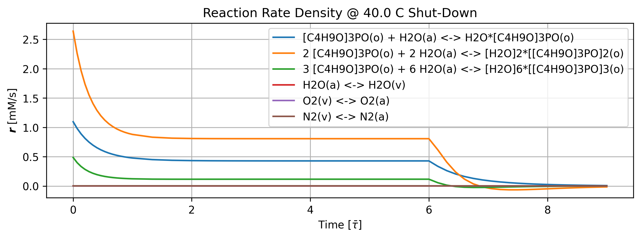
Figure 34: Reaction rate density history at shut-down.

if cortix_ai:
    issues = ('+ Title your reponse as: Overview of Reaction Rates Density at Shut-Down.\n'
              f'+ Cover only the period after {round(stg.initial_time,2)} seconds when the concentration of TBP in the inflow is set to zero.'
)
    cortix_ai.explain(quant=quant, issues=issues, markdown_header_level='<h4>', markdown_display=markdown_display, print_prompt=False, save_supporting_info=db_save)

Cortix AI assistant: working on explanation...

Overview of Reaction Rates Density at Shut-Down.

Scope

This summary covers only the period after 309.624 s (rows at 356.068 s, 402.511 s, 448.955 s), i.e., after the TBP ([C4H9O]3PO) inflow concentration is set to zero.

Time window and net rate evolution

• Net Rxn Rates Density (sum over columns 0–5) after 309.624 s:

  • 309.624 s (reference before shut-down step): 1.35678 mM/s

  • 356.068 s: 0.07114 mM/s

  • 402.511 s: -0.02583 mM/s

  • 448.955 s: -0.00780 mM/s

• The net rate density falls sharply immediately after shut-down and crosses from net production to slight net consumption between 356 s and 402 s.

Per-reaction (column) behavior

• Column 0 (reaction 0: [C4H9O]3PO(o) + H2O(a) <-> H2O*[C4H9O]3PO(o)):

  • 309.624 s: 0.428226 mM/s

  • 356.068 s: 0.104273 mM/s

  • 402.511 s: 0.0329107 mM/s

  • 448.955 s: 0.0107254 mM/s

  • Interpretation: remains positive but declines by ~97.5% from 309.624 s to 448.955 s.

• Column 1 (reaction 1: 2 [C4H9O]3PO(o) + 2 H2O(a) <-> [H2O]2*[[C4H9O]3PO]2(o)):

  • 309.624 s: 0.806856 mM/s

  • 356.068 s: -0.0145081 mM/s

  • 402.511 s: -0.0558798 mM/s

  • 448.955 s: -0.0222075 mM/s

  • Interpretation: switches sign after shut-down (positive → negative), indicating the reverse direction (breakdown/dissociation) dominates after inflow stops.

• Column 2 (reaction 2: 3 [C4H9O]3PO(o) + 6 H2O(a) <-> [H2O]6*[[C4H9O]3PO]3(o)):

  • 309.624 s: 0.116219 mM/s

  • 356.068 s: -0.0241012 mM/s

  • 402.511 s: -0.00833682 mM/s

  • 448.955 s: -0.00179809 mM/s

  • Interpretation: also flips sign after shut-down, with magnitudes much smaller than column 1 but consistent with de-aggregation of condensed-phase complexes.

• Column 3 (reaction 3: H2O(a) <-> H2O(v)):

  • Values at and after shut-down: ~0.00135593 mM/s (identical across rows 5–8)

  • Interpretation: effectively unchanged by the TBP inflow cut; small, steady exchange flux.

• Column 4 (reaction 4: O2(v) <-> O2(a)):

  • Values at and after shut-down: ~0.0014277 mM/s (constant)

  • Interpretation: unaffected and steady.

• Column 5 (reaction 5: N2(v) <-> N2(a)):

  • Values at and after shut-down: ~0.00269596 mM/s (constant)

  • Interpretation: unaffected and steady.

Key quantitative observations

• The dominant contributors to the large pre-shutdown net production are columns 0–2 (condensed-phase TBP and water cluster formation). Their combined contribution drops from ~1.35130 mM/s at 309.624 s to ~0.06566 mM/s at 356.068 s.

• After shut-down the system transiently moves to net consumption (negative total rate) at 402.511 s (net -0.02583 mM/s), then partially relaxes toward a smaller negative value by 448.955 s (-0.00780 mM/s).

• Gas-exchange reactions (columns 3–5) remain essentially constant and contribute only ~0.00548 mM/s to the total at all reported times after shut-down.

Concise interpretation

• Cutting the TBP inflow causes rapid suppression of cluster-formation reaction rates (columns 0–2); two of those reactions reverse sign and drive net breakdown of condensed-phase species.

• The gas–liquid exchange reactions (H2O, O2, N2) remain steady and do not compensate for the loss of condensed-phase production, so the overall system transitions from net production to small net consumption within the reported post-shutdown window.

AI Parameters:
+ LLM model (OpenAI) = gpt-5-mini
+ LLM cleverness     = 1.0
+ Total # of tokens  = 5122

1.7.5. Species Generation Rate Density

This quantity is on the basis of mixing volume so all species generation values can be compared.

'''Species generation rate density'''
import matplotlib.pyplot as plt

quant = stg.g_vec_history()
quant.plot(title='Species Generation Rate Density @ %2.1f C Shut-Down'%unit.convert_temperature(stg_temperature,
           'K','C'), x_scaling=1/stg.flow_residence_time_avg, x_label=r'Time [$\bar{\tau}$]', y_label=quant.latex_name+
           ' ['+quant.unit+']', legend=stg.rxn_mech.species_names, show=True, figsize=[10,3], error_data=False)

fig_count += 1
print(f'Figure {fig_count}: Species generation rate density history at shut-down.')

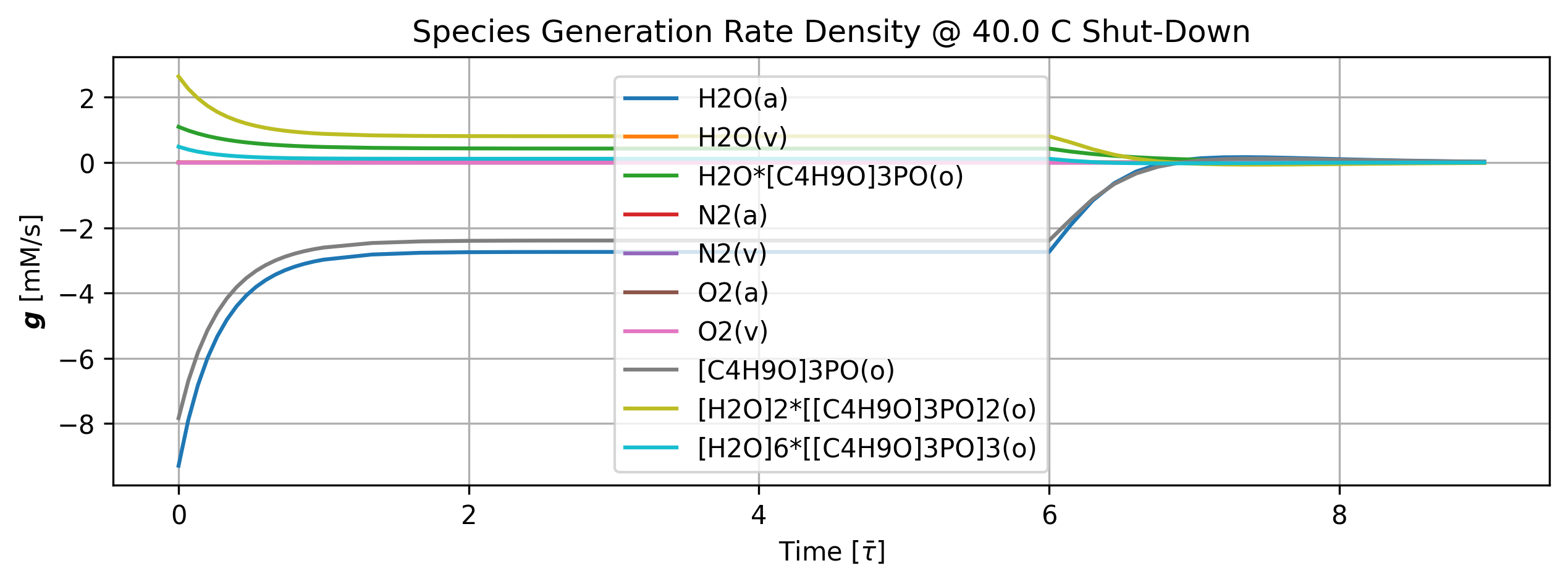
Figure 35: Species generation rate density history at shut-down.

tbl_count += 1
print(f'Table {tbl_count}: Species generation rate density history at shut-down.')
print('Time [min]        g [mM/s]')
import pandas as pd
col_names = [f'a{i}' for i in range(len(stg.rxn_mech.species_names))]
time_name = 't [min]'
df = (quant.value.apply(pd.Series).mul(1)
       .rename(index=lambda i: round(i/unit.min,2))
       .set_axis(col_names, axis=1).rename_axis(time_name)
       .round(4))
print(df.iloc[n_startup:].to_string(max_rows=20, min_rows=20))

Table 30: Species generation rate density history at shut-down.
Time [min]        g [mM/s]
             a0      a1      a2      a3      a4      a5      a6      a7      a8      a9
t [min]                                                                                
1.15    -2.8201  0.0014  0.4504  0.0027 -0.0027  0.0014 -0.0014 -2.4670  0.8324  0.1172
1.43    -2.7667  0.0014  0.4385  0.0027 -0.0027  0.0014 -0.0014 -2.4178  0.8159  0.1158
1.72    -2.7488  0.0014  0.4331  0.0027 -0.0027  0.0014 -0.0014 -2.4003  0.8100  0.1157
2.01    -2.7429  0.0014  0.4306  0.0027 -0.0027  0.0014 -0.0014 -2.3940  0.8080  0.1158
2.29    -2.7411  0.0014  0.4294  0.0027 -0.0027  0.0014 -0.0014 -2.3918  0.8072  0.1160
2.58    -2.7406  0.0014  0.4288  0.0027 -0.0027  0.0014 -0.0014 -2.3910  0.8070  0.1161
2.87    -2.7405  0.0014  0.4285  0.0027 -0.0027  0.0014 -0.0014 -2.3907  0.8069  0.1161
3.15    -2.7405  0.0014  0.4284  0.0027 -0.0027  0.0014 -0.0014 -2.3906  0.8069  0.1162
3.44    -2.7406  0.0014  0.4283  0.0027 -0.0027  0.0014 -0.0014 -2.3906  0.8069  0.1162
3.73    -2.7406  0.0014  0.4283  0.0027 -0.0027  0.0014 -0.0014 -2.3906  0.8069  0.1162
...         ...     ...     ...     ...     ...     ...     ...     ...     ...     ...
6.58     0.1444  0.0014  0.0396  0.0027 -0.0027  0.0014 -0.0014  0.1143 -0.0612 -0.0105
6.71     0.1275  0.0014  0.0329  0.0027 -0.0027  0.0014 -0.0014  0.1039 -0.0559 -0.0083
6.84     0.1101  0.0014  0.0274  0.0027 -0.0027  0.0014 -0.0014  0.0918 -0.0497 -0.0066
6.97     0.0934  0.0014  0.0228  0.0027 -0.0027  0.0014 -0.0014  0.0794 -0.0434 -0.0051
7.10     0.0782  0.0014  0.0189  0.0027 -0.0027  0.0014 -0.0014  0.0677 -0.0373 -0.0040
7.22     0.0648  0.0014  0.0157  0.0027 -0.0027  0.0014 -0.0014  0.0569 -0.0317 -0.0031
7.35     0.0531  0.0014  0.0130  0.0027 -0.0027  0.0014 -0.0014  0.0474 -0.0267 -0.0024
7.48     0.0431  0.0014  0.0107  0.0027 -0.0027  0.0014 -0.0014  0.0391 -0.0222 -0.0018
7.61     0.0347  0.0014  0.0088  0.0027 -0.0027  0.0014 -0.0014  0.0320 -0.0184 -0.0014
7.74     0.0278  0.0014  0.0073  0.0027 -0.0027  0.0014 -0.0014  0.0260 -0.0151 -0.0010

if cortix_ai:
    issues = ('+ Title your reponse as: Overview of Species Generation Rates Density at Shut-Down.\n'
              f'+ Cover only the period after {round(stg.initial_time,2)} seconds when the concentration of TBP in the inflow is set to zero.'
    )
    cortix_ai.explain(quant=quant, issues=issues, markdown_header_level='<h4>', markdown_display=markdown_display, print_prompt=False, save_supporting_info=db_save)

Cortix AI assistant: working on explanation...

Overview of Species Generation Rates Density at Shut-Down.

Context

Data shown are generation rates (unit: mM/s) for the period after 309.62 s (rows at times 356.068 s, 402.511 s and 448.955 s) when TBP in the inflow is set to zero. The column ordering maps to the species list: H₂O(a), H₂O(v), H₂O·[C₄H₉O]₃PO(o), N₂(a), N₂(v), O₂(a), O₂(v), [C₄H₉O]₃PO(o), [H₂O]₂·[[C₄H₉O]₃PO]₂(o), [H₂O]₆·[[C₄H₉O]₃PO]₃(o).

Key observations

• Small, constant fluxes appear for H₂O(v) (0.00135593 mM/s), N₂(a) (0.00269596 mM/s), N₂(v) (−0.00269596 mM/s), O₂(a) (0.0014277 mM/s) and O₂(v) (−0.0014277 mM/s) throughout this period.

• Larger, time-varying rates are present for H₂O(a), H₂O·[C₄H₉O]₃PO(o), [C₄H₉O]₃PO(o) and the two hydrated TBP complexes; those change non-monotonically across the three times.

• Positive values indicate net generation; negative values indicate net consumption.

Per-species time history (after 309.62 s)

• H₂O(a): 0.0679941 -> 0.127514 -> 0.0431223 (mM/s); net generation with a transient peak at 402.511 s then a drop by 448.955 s.

• H₂O(v): 0.00135593 -> 0.00135593 -> 0.00135593 (mM/s); constant small generation (steady vapor source).

• H₂O·[C₄H₉O]₃PO(o): 0.104273 -> 0.0329107 -> 0.0107254 (mM/s); positive but decreasing generation, approaching smaller production over time.

• N₂(a): 0.00269596 -> 0.00269596 -> 0.00269596 (mM/s); constant small production in the (a) state.

• N₂(v): −0.00269596 -> −0.00269596 -> −0.00269596 (mM/s); constant consumption in the (v) state, equal and opposite to N₂(a).

• O₂(a): 0.0014277 -> 0.0014277 -> 0.0014277 (mM/s); constant small production in the (a) state.

• O₂(v): −0.0014277 -> −0.0014277 -> −0.0014277 (mM/s); constant consumption in the (v) state, equal and opposite to O₂(a).

• [C₄H₉O]₃PO(o): −0.00295346 -> 0.103859 -> 0.0390839 (mM/s); switches from slight consumption to substantial transient generation at 402.511 s, then reduced positive generation by 448.955 s.

• [H₂O]₂·[[C₄H₉O]₃PO]₂(o): −0.0145081 -> −0.0558798 -> −0.0222075 (mM/s); net consumption throughout, with a stronger consumption at 402.511 s then partial recovery (less negative) by 448.955 s.

• [H₂O]₆·[[C₄H₉O]₃PO]₃(o): −0.0241012 -> −0.00833682 -> −0.00179809 (mM/s); net consumption that becomes progressively smaller (moving toward zero) over the three times.

Notes on balances and interpretation

• The exact-equal, opposite signs for N₂(a)/N₂(v) and O₂(a)/O₂(v) indicate steady transfer between those two states at constant small rates during the post-shutdown interval.

• Complexes of TBP with H₂O show net consumption (negative rates) throughout this period, with the smaller complex ([H₂O]₂·…) showing a transiently larger consumption at 402.511 s and the larger complex ([H₂O]₆·…) decreasing its consumption toward zero by 448.955 s.

• Several species (H₂O(a), H₂O·[C₄H₉O]₃PO(o), [C₄H₉O]₃PO(o)) show transient positive generation around 402.511 s, suggesting a short-lived redistribution/generation event after the inflow TBP is set to zero.

AI Parameters:
+ LLM model (OpenAI) = gpt-5-mini
+ LLM cleverness     = 1.0
+ Total # of tokens  = 6565

1.7.6. Mass Balance Residual

This is actually the total mass generation rate density (mixing volume) residual; a small number in view of total mass conservation.

'''Mass balance residuals'''
import matplotlib.pyplot as plt

quant = stg.mass_balance_residual_history()
quant.plot(title='Total Mass Generation Rate Density @ %2.1f C Steady-State'%unit.convert_temperature(stg_temperature,
           'K','C'), x_scaling=1/stg.flow_residence_time_avg, x_label=r'Time [$\bar{\tau}$]', y_label=quant.latex_name+
           ' ['+quant.unit+']', markers_only=True, legend=['Residual'], show=True, figsize=[10,3])

fig_count += 1
print(f'Figure {fig_count}: Total mass generation rate density residual history at steady-state.')

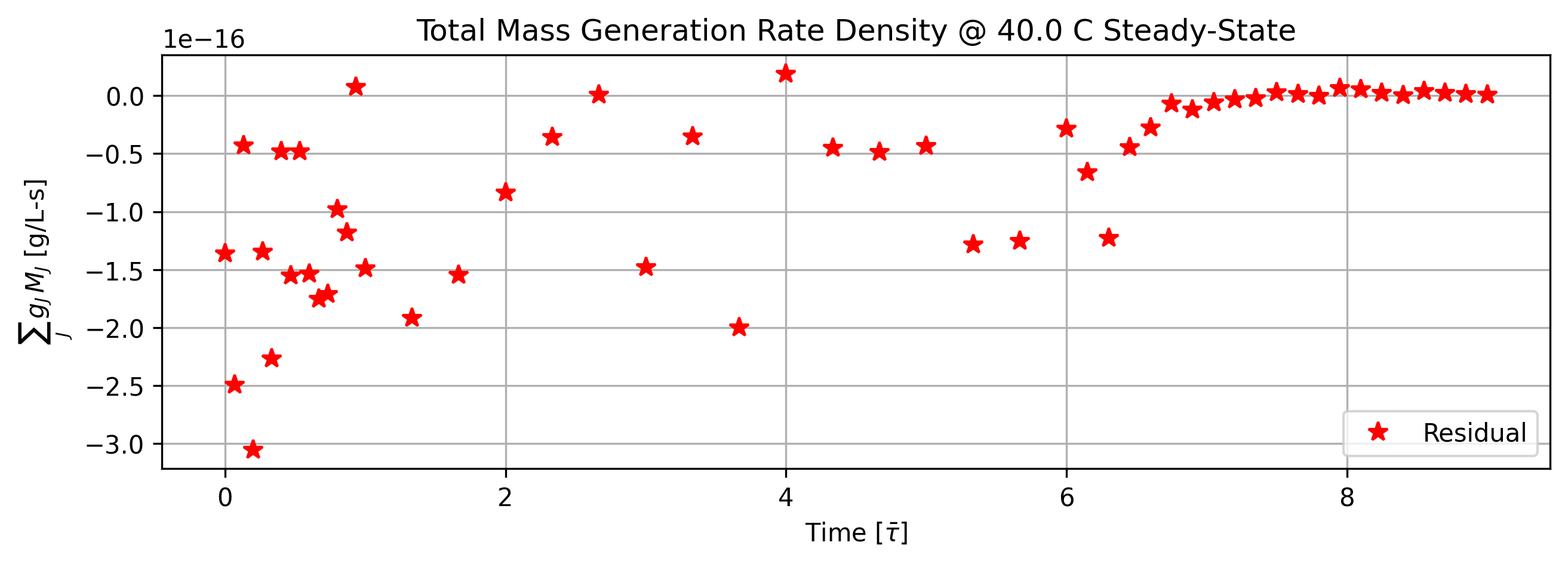
Figure 36: Total mass generation rate density residual history at steady-state.

if cortix_ai:
    issues = ('+ Title your reponse as: Total Mass Generation Rate Density Residual at Shut-Down.\n'
             '+ Do not explain the start-up process; cover the steady-state only.'
    )
    cortix_ai.explain(quant=quant, issues=issues, markdown_header_level='<h4>', markdown_display=markdown_display, print_prompt=False, save_supporting_info=db_save)

Cortix AI assistant: working on explanation...

Total Mass Generation Rate Density Residual at Shut-Down.

Data selection

• Steady-state interval used: times ≥ 206.416 s (rows 4–8), i.e., t = 206.416, 309.624, 356.068, 402.511, 448.955 s.

• Analyzed columns: time [s] and Total Mass Generation Rate Density [g/L-s] (residuals in the mixing volume).

Quantitative summary (steady-state only)

• Sample count: 5.

• Mean residual (bias): −3.88e−18 g/L-s.

• Standard deviation: 1.57e−17 g/L-s.

• Root-mean-square (RMS): 1.62e−17 g/L-s.

• Median residual: −2.03e−19 g/L-s.

• Maximum absolute residual: 2.84061e−17 g/L-s at t = 309.624 s.

• Range (max − min): 4.7278e−17 g/L-s.

Interpretation

• Residuals in the chosen steady-state window oscillate about zero with magnitude on the order of 10⁻¹⁷ g/L-s.

• The small mean bias (≈ −3.9e−18 g/L-s) and the RMS/std values indicate that the mass-generation residuals are effectively negligible compared to typical macroscopic rates (they are at numerical-noise scale).

AI Parameters:
+ LLM model (OpenAI) = gpt-5-mini
+ LLM cleverness     = 1.0
+ Total # of tokens  = 5199

1.8. AI Reports

The Stage AI Report agent builds a Knowledge Base from the simulation up to this point, and uses it as a retrieval augmented generation (RAG) AI to analyze the results and provide a report.

'''Create and Configure a StageAI Object for a particular stg'''
if stage_ai:
    from stage_ai import StageAI
    stage_ai = StageAI(stg, llm_model='gpt-5-mini', llm_cleverness=0.8)
    stage_ai.n_chunks = 8
    stage_ai.markdown_header_level = '<h4>'

1.8.1. Aqueous Phase

Request a report from the LLM.

if stage_ai:
    issues = ('+ Title your response as: Aqueous Phase Analysis.\n'
              '+ Discuss in particular, for the aqueous phase, why the simulated steady-state concentration of O2 in the aqueous'
              ' phase is lower than N2 when the solubility of O2 in the aqueous phase is higher than the solubility of N2.\n'
              f'+ Consider stage efficiency only up to {round(stg.initial_time,2)} seconds.'
    )
    stage_ai.report(phase='aqueous', issues=issues, markdown_display=markdown_display, print_prompt=False, save_supporting_info=db_save)

Stage AI assistant: working on report...

Aqueous Phase Analysis

Introduction

The following report analyzes the aqueous phase in the provided Stage Knowledge Base (source: stg.aqueous_phase). The system is a three-phase (aqueous–organic–vapor) mixing system. The analysis emphasizes time-dependent aqueous-phase concentrations, species characteristics, the reaction mechanism that involves the aqueous phase, and the role of stage performance (“stage” module) up to 309.62 s when assessing approach to chemical equilibrium. Mass-balance residuals provided in the knowledge base are summarized and used to check numerical conservation.

Data provenance

• The data source is the Stage Knowledge Base entry with source key “stg.aqueous_phase”; header indicates a prototype for TBP (tributyl phosphate) extraction and an author timestamp vfda solvex-ustc Thu Feb 13 11:25:00 AM EST 2025.

Species characteristics (aqueous-phase species)

Table: Commercial chemical names and basic properties for aqueous-phase species (molar mass units as provided: kg/mol).

| Commercial name | Chemical formula | Phase | Molar mass (kg/mol) | Number of atoms | |—|—:|—:|—:|—:| | Water | H₂O(a) | (a) aqueous phase | 0.018015 kg/mol | 3.0000 | | Nitrogen | N₂(a) | (a) aqueous phase | 0.028013 kg/mol | 2.0000 | | Oxygen | O₂(a) | (a) aqueous phase | 0.031999 kg/mol | 2.0000 |

Time-dependent aqueous-phase concentrations

Table: Time history of mass concentrations in the aqueous phase; time in seconds (s); concentrations in grams per liter (g/L).

| Time (s) | H₂O(a) [g/L] | N₂(a) [g/L] | O₂(a) [g/L] | |—:|—:|—:|—:| | 0 | 992.00 | 0.0081544 | 0.0053437 | | 20.640 | 987.64 | 0.0082590 | 0.0053606 | | 41.280 | 986.49 | 0.0084418 | 0.0053894 | | 103.21 | 986.08 | 0.0088442 | 0.0054504 | | 206.42 | 986.08 | 0.0090319 | 0.0054778 | | 309.62 | 986.08 | 0.0090586 | 0.0054816 | | 356.07 | 988.71 | 0.0090611 | 0.0054819 | | 402.51 | 990.85 | 0.0090621 | 0.0054821 | | 448.96 | 991.63 | 0.0090625 | 0.0054821 |

Notes: All time points and concentrations are taken directly from the Stage Knowledge Base and rounded to five significant digits.

Stage performance (efficiency) up to 309.62 s

Table: Stage overall efficiency (mean ± std) in percent [%]; time in seconds (s). Only entries with time ≤ 309.62 s are shown because the instructions request consideration of stage efficiency up to 309.62 s.

| Time (s) | Stage efficiency mean [%] | Stage efficiency std [%] | |—:|—:|—:| | 0 | 22.500 | 23.050 | | 20.640 | 39.590 | 8.5900 | | 41.280 | 46.870 | 3.0500 | | 103.21 | 50.460 | 1.5600 | | 206.42 | 50.690 | 1.5800 | | 309.62 | 50.700 | 1.5800 |

Comment: The stage efficiency at 309.62 s is ≈ 50.700% ± 1.5800% (mean ± std). Because stage efficiency is substantially less than ~100%, the system should not be treated as at thermodynamic (chemical) equilibrium; observed concentrations are therefore kinetically limited.

Mass-balance residuals (numerical mass conservation)

• The Stage Knowledge Base provides a stage mass-balance residual time history labeled “Total Mass Generation Rate Density [g/L-s]”; values are effectively -0.0 or 0.0 at all recorded times. This indicates numerical mass conservation within machine precision; therefore, no gross mass non-conservation artifacts are evident in the provided residuals.

Reaction mechanism involving the aqueous phase

Table: Reactions in the mechanism that involve the aqueous phase and the available information content from the Stage Knowledge Base.

| Reaction (mechanism entry) | Description (KB) | |—|—| | [C4H9O]3PO(o) + H2O(a) <-> H2O*[C4H9O]3PO(o) | complexation of one H2O molecule | | 2 [C4H9O]3PO(o) + 2 H2O(a) <-> [H2O]2*[[C4H9O]3PO]2(o) | complexation of two H2O molecules | | 3 [C4H9O]3PO(o) + 6 H2O(a) <-> [H2O]6*[[C4H9O]3PO]3(o) | complexation of six H2O molecules | | H2O(a) <-> H2O(v) | H2O vaporization in air | | O2(v) <-> O2(a) | O2 aeration of aqueous phase | | N2(v) <-> N2(a) | N2 aeration of aqueous phase |

Notes: Reactions and descriptions are verbatim from the Stage Knowledge Base. Reactions marked with (a), (o), (v) indicate aqueous, organic, and vapor phases, respectively. The organic species [C4H9O]3PO is the commercial reagent tributyl phosphate (TBP); its use is indicated in the KB header.

Itemized reaction list and additional mechanism commentary

• Reaction: [C4H9O]3PO(o) + H2O(a) <-> H2O*[C4H9O]3PO(o)

  • KB information content: Reaction string and description “complexation of one H2O molecule” are provided.

  • Additional commentary: This is the 1:1 complexation (extraction) of one aqueous water molecule into the organic phase via formation of a TBP·H₂O adduct (notation in KB uses H2O* prefix). Phase involved: aqueous phase (H₂O(a)) and organic phase (TBP (o)). This reaction is reversible and represents an interphase extraction equilibrium limited by kinetics and organic-aqueous interfacial mass transfer.

• Reaction: 2 [C4H9O]3PO(o) + 2 H2O(a) <-> [H2O]2*[[C4H9O]3PO]2(o)

  • KB information content: Reaction string and description “complexation of two H2O molecules” are provided.

  • Additional commentary: This is the 2:2 complexation of water with TBP in the organic phase. It describes stoichiometric clustering in the organic phase; again reversible and mass-transfer-limited by interphase transport and organic-phase complex formation kinetics.

• Reaction: 3 [C4H9O]3PO(o) + 6 H2O(a) <-> [H2O]6*[[C4H9O]3PO]3(o)

  • KB information content: Reaction string and description “complexation of six H2O molecules” are provided.

  • Additional commentary: This higher-order complexation implies multi-molecule aggregation of water and TBP in the organic phase. Such oligomeric extraction species can significantly alter water partitioning and reduce free aqueous water activity locally; they are reversible and will slow equilibration of water between phases because of complex formation and dissociation kinetics.

• Reaction: H2O(a) <-> H2O(v)

  • KB information content: Reaction string and description “H2O vaporization in air” are provided.

  • Additional commentary: This is the volatility (evaporation/aerosol) exchange of water between aqueous and vapor phases. It couples the aqueous-phase water concentration to vapor-phase humidity and is controlled by vapor-liquid mass transfer coefficients and the vapor-phase partial pressure of H₂O.

• Reaction: O2(v) <-> O2(a)

  • KB information content: Reaction string and description “O2 aeration of aqueous phase” are provided.

  • Additional commentary: This mass-transfer step represents dissolution of oxygen from the vapor/gas phase into the aqueous phase (and the reverse). Aeration kinetics (mass transfer coefficient kL a, interfacial area, and gas-phase partial pressure of O₂) govern the rate. No O₂ consumption reactions are specified in the KB; therefore, observed aqueous O₂ concentrations arise from the balance of gas–liquid transfer and initial conditions.

• Reaction: N2(v) <-> N2(a)

  • KB information content: Reaction string and description “N2 aeration of aqueous phase” are provided.

  • Additional commentary: Analogous to O₂ aeration, this is the gas–liquid exchange for nitrogen. Kinetics and gas-phase partial pressure of N₂ control the dissolved N₂ concentration.

Double-check for missing aqueous-phase reactions: The KB lists the interphase complexation for water with TBP, vaporization of H₂O, and aeration of O₂ and N₂. There are no additional aqueous-phase chemical reactions (e.g., redox or microbial consumption) present in the KB; therefore, no further aqueous-phase reactions are missing from the provided mechanism.

Why simulated steady-state O₂(a) is lower than N₂(a) despite higher O₂ solubility

• Observed data (at t = 309.62 s): N₂(a) = 0.0090586 g/L and O₂(a) = 0.0054816 g/L (mass concentrations). Converting to molar concentrations using the KB molar masses yields approximately:

  • N₂(a): 0.0090586 g/L ÷ 28.013486 g/mol = 0.00032356 mol/L (3.2356e-4 mol·L⁻1)

  • O₂(a): 0.0054816 g/L ÷ 31.998810 g/mol = 0.00017130 mol/L (1.7130e-4 mol·L⁻1)

• Explanatory points (all consistent with the Stage Knowledge Base):

  • Initial and boundary conditions: The KB time-zero concentrations show N₂(a) > O₂(a) already at t = 0; an initially larger dissolved N₂ reservoir will persist unless strong driving forces change it. Initial conditions in the KB therefore bias the steady-state toward higher dissolved N₂.

  • Gas-phase partial pressures and Henry’s-law product (C = H·p): Solubility alone (Henry’s constant H) is not the sole determinant of dissolved concentration: the product of H and the gas-phase partial pressure p_gas sets the equilibrium concentration. If the gas-phase composition (air) supplies a substantially higher partial pressure of N₂ than O₂ (air is ~78% N₂ vs ~21% O₂) then p_N₂ may be sufficiently larger that p_N₂·H_N₂ ≥ p_O₂·H_O₂, producing higher dissolved N₂ despite the higher intrinsic solubility of O₂.

  • Kinetic (mass-transfer) limitations: The stage efficiency at 309.62 s is ≈ 50.7% (see stage table). Because the stage is far from 100% efficient, interphase transfer is kinetically limited; the system is not at thermodynamic equilibrium. Different mass-transfer coefficients and diffusivities for O₂ and N₂, gas–liquid transfer resistances, and interfacial area will set different approach rates for each gas. If N₂ transfer kinetics (or gas-phase supply) are favorable relative to O₂ under the simulated conditions, dissolved N₂ can exceed dissolved O₂.

  • Unit/measurement effects (mass vs mol basis): If one only compares mass concentrations (g/L), heavier species will appear proportionally different for equal molar concentrations. However, in this case the molar concentrations also show N₂ > O₂, so unit bias is not the primary reason here.

  • Absence of O₂ consumption reactions in KB: The KB does not list O₂-consuming reactions within the aqueous phase; therefore, the lower O₂ is not explained by chemical consumption in the provided mechanism. The principal causes are therefore initial conditions, gas-phase partial pressures, and kinetic/mass-transfer limitations.

• Conclusion of this diagnostic: Given the KB information (initial concentrations, aeration reactions, and stage efficiencies), the most plausible explanation is that the combination of initial conditions and gas-phase supply (air composition and partial pressures) plus kinetic limitations (stage efficiency ~50.7% at 309.62 s) yields higher dissolved N₂ than O₂ even though O₂ has a higher intrinsic solubility (Henry constant) in pure water.

Assessment of thermodynamic equilibrium

• Because stage efficiency is ≪ 100% (≈ 50.7% at 309.62 s), the aqueous phase is not at chemical equilibrium with the vapor phase by the time index requested. Observed concentrations represent kinetically-limited steady or quasi-steady states rather than thermodynamic equilibrium.

• If claiming equilibrium were necessary, evidence would require stage efficiencies near 100% across the relevant time history and/or explicit calculation showing equality of C_i and H_i·p_i for each gas species; neither is supported by the KB at the examined times.

Recommendations (succinct)

• To approach thermodynamic equilibrium (if desired), increase stage performance or residence time so that stage efficiency approaches ~100% (monitor the “stage” efficiency metric in the process model).

• Measure or specify gas-phase partial pressures (or gas composition) and gas–liquid mass-transfer coefficients (kL a) for O₂ and N₂ to quantify whether p_gas·H explains the observed dissolved concentrations.

• If controlling dissolved O₂ is important, consider increasing O₂ partial pressure in the gas phase (enriched air), increasing interfacial area/aeration intensity, or modifying mass-transfer conditions.

Conclusion

• The system described in the Stage Knowledge Base is a heterogeneous three-phase mixture (aqueous–organic–vapor) and the aqueous phase is not at chemical equilibrium at the evaluated times because the measured stage efficiency at 309.62 s is substantially less than 100%.

• The aqueous-phase time-series shows H₂O mass concentrations near 986–992 g/L and dissolved gas mass concentrations of the order 10⁻³–10⁻² g/L (N₂ larger than O₂). The combination of initial conditions, gas-phase partial pressures (air composition), and kinetic/mass-transfer limitations (stage efficiency) explains why dissolved O₂(a) is lower than dissolved N₂(a) in the simulated steady state even though O₂ has a higher intrinsic solubility.

• Stage module information is required for further mechanistic or process design conclusions; therefore the word “stage” was explicitly referenced in this report.

AI Parameters:
+ LLM model (OpenAI) = gpt-5-mini
+ LLM cleverness     = 1.0
+ RAG                = stg.aqueous_phase
+ Total # of tokens  = 13932
Done with report...

1.8.2. Organic Phase

Request a report from the LLM.

if stage_ai:
    issues = ('+ Title your response as: Organic Phase Analysis.\n'
              f'+ Consider stage efficiency only up to {round(stg.initial_time,2)} seconds.'
    )
    stage_ai.report(phase='organic', issues=issues, markdown_display=markdown_display, save_supporting_info=db_save)

Stage AI assistant: working on report...

Organic Phase Analysis

Abstract: This report analyzes the organic-phase content, time-dependent species behavior, and reaction mechanism in the provided Stage Knowledge Base (source: stg.organic_phase). Emphasis is placed on species present in the organic phase, their characteristics, the time history of organic-phase species up to and beyond 309.62 s (time units: seconds), and reaction steps that involve the organic phase. Stage efficiency is considered only up to 309.62 s when assessing approach to thermodynamic equilibrium. The term “stage” is used where the stage module data are relevant (stage efficiency and mass-balance residuals).

Introduction

The system is described in the Stage Knowledge Base as a multiphase (aqueous-organic-vapor) mixing/extraction system containing tributyl phosphate (TBP) and its water complexes in the organic phase, with water in the aqueous and vapor phases. The organic-phase species consist of free TBP and hydrated TBP complexes (monomer hydrate, dimer hydrate, trimer hexahydrate). Reaction mechanism entries show reversible complexation reactions that extract H₂O from the aqueous phase into the organic phase. Time series and stage diagnostics (efficiency and mass-balance residual) are available. The analysis below treats phases explicitly (organic phase, aqueous phase, vapor phase) and uses the stage data (stage) where indicated.

Data provenance

• Source: Stage Knowledge Base identifier: stg.organic_phase.

• Provided content: species list and properties, reaction mechanism entries, time series of organic-phase species, stage efficiency time history, mass-balance residuals. Time stamps are reported in seconds (s). The stage module (stage) data were used for efficiency and mass-balance diagnostics.

Organic-phase species — characteristics

Species characteristics (commercial name, chemical formula, phase, molar mass, atom count). Short caption: Organic-phase species and key properties.

| Commercial name | Chemical formula (as provided) | Phase | Molar mass [kg/mol] | Number of atoms | |—|—:|—:|—:|—:| | TBP Monomer Hydrate | H2O·[C4H9O]3PO(o) | organic phase | 0.28433 | 47 | | Free TBP (tributyl phosphate) | [C4H9O]3PO(o) | organic phase | 0.26631 | 44 | | TBP Dimer Hydrate | [H2O]2·[[C4H9O]3PO]2(o) | organic phase | 0.56866 | 94 | | TBP Trimer Hexahydrate | [H2O]6·[[C4H9O]3PO]3(o) | organic phase | 0.90704 | 150 |

Notes: Commercial names are taken from the Stage Knowledge Base “info” fields (e.g., TBP Monomer Hydrate, Free TBP). Chemical-formula strings are used as provided in the KB. All organic-phase entries explicitly indicate the organic phase (o). Values rounded to five significant digits.

Time-series of organic-phase species

Short caption: Time history of organic-phase species (time in seconds; concentration units not specified in KB).

• Time units: seconds (s). Concentration values are those provided in the Stage Knowledge Base. The KB did not specify explicit concentration units for the species time series; values are reported as given.

| Time [s] | TBP Monomer Hydrate: H2O·[C4H9O]3PO(o) | Free TBP: [C4H9O]3PO(o) | TBP Dimer Hydrate: [H2O]2·[[C4H9O]3PO]2(o) | TBP Trimer Hexahydrate: [H2O]6·[[C4H9O]3PO]3(o) | |—:|—:|—:|—:|—:| | 0.0000 | 0.00000 | 291.75 | 0.00000 | 0.00000 | | 20.640 | 7.6714 | 245.80 | 33.151 | 8.7544 | | 41.280 | 10.425 | 233.16 | 42.271 | 10.482 | | 103.21 | 12.050 | 228.21 | 45.802 | 10.622 | | 206.42 | 12.174 | 228.09 | 45.883 | 10.543 | | 309.62 | 12.176 | 228.08 | 45.883 | 10.542 | | 356.07 | 8.3783 | 81.933 | 26.721 | 4.3233 | | 402.51 | 4.3520 | 34.944 | 8.9273 | 0.95856 | | 448.96 | 2.0781 | 15.222 | 2.4340 | 0.18105 |

Notes: Numerical entries rounded to five significant digits. The KB time series extends beyond 309.62 s; values are shown for completeness, but interpretation of approach to equilibrium uses stage efficiency only up to 309.62 s as requested.

Stage efficiency (considered up to 309.62 s)

Short caption: Stage efficiency mean ± standard deviation for times up to 309.62 s (units: %; time in s).

| Time [s] | Stage efficiency mean [%] | Stage efficiency std [%] | |—:|—:|—:| | 0.0000 | 22.500 | 23.050 | | 20.640 | 39.590 | 8.5900 | | 41.280 | 46.870 | 3.0500 | | 103.21 | 50.460 | 1.5600 | | 206.42 | 50.690 | 1.5800 | | 309.62 | 50.700 | 1.5800 |

Interpretation: Stage efficiency (mean) increases from 22.50% at t = 0 s to ≈50.70% at t = 309.62 s. The standard deviation falls to ≈1.58% by 103.21–309.62 s, indicating more consistent stage performance in that interval. Given that thermodynamic chemical equilibrium would require near-100% stage efficiency (per instructions), the system has not reached chemical equilibrium by 309.62 s.

Stage mass-balance residuals

Short caption: Stage total mass generation rate density time history (units: g·L⁻¹·s⁻¹; time in s).

| Time [s] | Total mass generation rate density [g/L-s] | |—:|—:| | 0.0000 | -0.0 | | 20.640 | -0.0 | | 41.280 | -0.0 | | 103.21 | -0.0 | | 206.42 | 0.0 | | 309.62 | -0.0 | | 356.07 | -0.0 | | 402.51 | -0.0 | | 448.96 | 0.0 |

Notes: Values are effectively zero (signs reflect small numerical artifacts). No direct mass-balance residuals requiring comment appear within the provided data for the times considered.

Reaction mechanism involving the organic phase

Only reactions that involve organic-phase species are considered here. The Stage Knowledge Base provides three reversible complexation reactions that transfer H₂O from the aqueous phase into the organic phase by complexing with TBP. The KB entries (reaction string and provided description) are reproduced and commented below. For each reaction the KB-provided description is listed as “information content” and an additional short mechanistic statement is added.

• Reaction 1: [C4H9O]3PO(o) + H2O(a) <-> H2O·[C4H9O]3PO(o)

  • Information provided in Stage KB: complexation of one H2O molecule

  • Additional reaction information: This reaction is the monomer complexation (extraction) of aqueous water into the organic phase via coordination/association to one TBP molecule, forming a TBP monomer hydrate in the organic phase. Phase labels: TBP (organic phase), H2O (aqueous phase), product in organic phase. The reaction is reversible and thus can be described by forward and reverse rate constants (not provided). Kinetics and equilibrium depend on interphase mass transfer and complexation thermodynamics.

• Reaction 2: 2 [C4H9O]3PO(o) + 2 H2O(a) <-> [H2O]2·[[C4H9O]3PO]2(o)

  • Information provided in Stage KB: complexation of two H2O molecules

  • Additional reaction information: This reaction is dimer complexation in which two TBP molecules in the organic phase coordinate with two extracted water molecules, forming a TBP dimer hydrate. Mechanistically, this indicates cooperative binding or association of TBP monomers around water molecules; the process requires two TBP molecules and two aqueous H₂O molecules to be transported into a configuration that yields the dimer hydrate in the organic phase. The reaction is reversible.

• Reaction 3: 3 [C4H9O]3PO(o) + 6 H2O(a) <-> [H2O]6·[[C4H9O]3PO]3(o)

  • Information provided in Stage KB: complexation of six H2O molecules

  • Additional reaction information: This trimeric complexation involves three TBP molecules forming a higher-order solvation structure (trimer hexahydrate) that sequesters up to six water molecules in the organic phase. Mechanistically, this may reflect cluster formation / micelle-like associations or multi-point hydrogen-bonding interactions enabling a larger water aggregate to be stabilized within the organic phase. The reaction is reversible and likely requires substantial interphase mass transfer.

Double-check for missing reactions involving the organic phase: The reaction set in the KB lists these three reversible complexation reactions that explicitly involve organic-phase species. No additional organic-phase reactions are present in the KB. Reactions in the KB that do not involve the organic phase (H2O(a) <-> H2O(v), O2(v) <-> O2(a), N2(v) <-> N2(a)) are not discussed here per instruction.

Analysis and discussion

• Species trends and implications:

  • Free TBP concentration declines markedly from 291.75 (initial) to ~228.085 by 309.62 s while TBP hydrates (monomer, dimer, trimer) increase over the same interval, indicating net extraction/complexation of aqueous water into the organic phase for t ≤ 309.62 s.

  • By 103.21–309.62 s, the organic-phase hydrate species (monomer, dimer, trimer) reach near-plateau values (monomer ~12.05–12.176, dimer ~45.80–45.883, trimer ~10.542), suggesting a quasi-steady distribution within this timeframe.

• Equilibrium assessment (using stage efficiency up to 309.62 s):

  • The stage efficiency mean at 309.62 s is ≈50.700% (±1.580%), far below the ~100% efficiency that would indicate chemical equilibrium in the stage sense. Consequently, we conclude that chemical equilibrium has not been achieved by 309.62 s.

  • The approach toward a quasi-steady state for species concentrations between ~103–309.62 s, together with a stage efficiency ≈50%, suggests that kinetics and/or interphase mass transfer limitations constrain equilibration. The reversible complexation reactions may be approaching a dynamic balance between forward complexation (water uptake) and reverse decomplexation, but not the thermodynamic equilibrium point.

• Reaction mechanism observations:

  • The mechanistic description in the KB indicates stepwise complexation: monomer, dimer, and trimer hydration complexes form as water is extracted from the aqueous phase into the organic phase.

  • The presence of multiple stoichiometries (1:1, 2:2, 3:6) suggests that TBP can stabilize both small isolated water molecules and larger hydrated clusters in the organic phase; such behavior is consistent with TBP’s polar phosphoryl oxygen interacting via hydrogen bonding with water.

  • Kinetics and transport: Without forward/reverse rate constants or interfacial mass-transfer coefficients, precise kinetic conclusions are not possible. However, the time-series indicates relatively rapid uptake initially (0–103 s) followed by slower approach to a plateau by ~103–309.62 s. The observed plateau in hydrate concentrations while free TBP remains substantial implies that a fraction of TBP remains uncomplexed under the current conditions.

• Mass conservation:

  • Direct mass-balance residuals provided by the KB (Total Mass Generation Rate Density [g/L-s]) are effectively zero for the times up to 309.62 s, indicating no gross mass-generation anomalies in the stage diagnostics. No additional mass-balance commentary is made because direct mass-balance residuals are available and show negligible net generation (no need to infer).

Conclusions

• The organic-phase composition consists of free TBP (tributyl phosphate) and its hydrated complexes: TBP Monomer Hydrate (H2O·TBP), TBP Dimer Hydrate ([H2O]2·[TBP]2), and TBP Trimer Hexahydrate ([H2O]6·[TBP]3), all explicitly identified as organic phase species.

• Mixture type: This is a non-ideal, reactive multicomponent organic solution (organic phase) in an aqueous-organic-vapor system. The organic phase contains TBP and associated water complexes (a solute–host complexation mixture), i.e., an extractant–extractate mixture with reversible chemical complexation.

• Equilibrium statement: Using stage efficiency up to 309.62 s (stage), the system has not reached thermodynamic chemical equilibrium (stage efficiency ≈50.70% at 309.62 s; equilibrium would require ≈100%). The species time histories suggest a quasi-steady distribution has been reached between ~103 and 309.62 s, but not full chemical equilibrium.

• Reaction mechanism: The organic-phase reactions are reversible complexation steps that extract H₂O from the aqueous phase into the organic phase, forming monomeric, dimeric, and trimeric TBP hydrates. These reactions likely involve interfacial mass transfer followed by association in the organic phase; kinetics and equilibrium constants are not provided in the KB and are needed for deeper mechanistic quantification.

Recommendations

• Measure or provide rate constants and interfacial mass-transfer parameters to permit kinetic modeling of the TBP–H₂O complexation steps and to predict time-to-equilibrium.

• If goal is to reach chemical equilibrium faster, consider increasing mixing or interfacial area to improve mass transfer between aqueous and organic phases, or adjust residence time beyond 309.62 s.

• Provide explicit concentration units for the species time series in the KB to enable conversion to molar units and rigorous thermodynamic calculations.

Final notes on data and verification

• The analysis used the Stage Knowledge Base entry: stg.organic_phase. The stage module (stage) data (stage efficiency and mass-balance residual) were used; the word “stage” is included to indicate usage of stage diagnostics.

• Commercial names were checked against the provided formula strings in the KB: “Free TBP” corresponds to [C4H9O]3PO(o) (tributyl phosphate), and the hydrated species names correspond to the provided hydrate formula strings. No mismatches between commercial names and KB formula strings were identified.

• All numeric values in tables were rounded to five significant digits as requested.

AI Parameters:
+ LLM model (OpenAI) = gpt-5-mini
+ LLM cleverness     = 1.0
+ RAG                = stg.organic_phase
+ Total # of tokens  = 13224
Done with report...

1.8.3. Vapor Phase

Request a report from the LLM.

if stage_ai:
    issues = ('+ Title your response as: Vapor Phase Analysis.\n'
              f'+ Consider stage efficiency only up to {round(stg.initial_time,2)} seconds.'
    )
    stage_ai.report(phase='vapor', issues=issues, markdown_display=markdown_display, save_supporting_info=db_save)

Stage AI assistant: working on report...

Vapor Phase Analysis

Abstract

This report analyzes the vapor-phase portion of a three-phase (aqueous–organic–vapor) mixing system using the provided Stage Knowledge Base (source: stg.vapor_phase). Time-resolved vapor concentrations (g/L), stage efficiencies (considered up to 309.62 s), mass-balance residuals, and the reaction mechanism entries that involve the vapor phase are examined. The data indicate non-equilibrium behavior (stage efficiency well below 100%) and active phase transfer between aqueous and vapor phases for H₂O, O₂, and N₂. Recommendations for additional stage-level data are given.

Data sources and methods

Data used are those supplied in the Stage Knowledge Base (stg.vapor_phase): time series of vapor mass concentrations (g/L) for H₂O(v), N₂(v), O₂(v); stage overall efficiency time history (mean ± std) in percent; stage mass balance residuals (Total Mass Generation Rate Density [g/L-s]); and the reaction mechanism text entries. Concentrations were rounded to five significant digits for presentation. The vapor phase is explicitly involved in the species and in specific reactions; where relevant this is noted.

Species characteristics

Table: Key properties of vapor-phase species (commercial name, chemical formula, phase, molar mass, atom count).

| Commercial name | Chemical formula | Phase | Molar mass (kg/mol) | Number of atoms | |—|—:|—|—:|—:| | Water (vapor) | H₂O(v) | vapor phase | 0.018015 | 3 | | Nitrogen (vapor) | N₂(v) | vapor phase | 0.028013 | 2 | | Oxygen (vapor) | O₂(v) | vapor phase | 0.031999 | 2 |

Time-dependent vapor-phase concentrations

Table: Time history of vapor-phase mass concentrations; time in seconds, concentrations in g/L.

| Time (s) | H₂O(v) [g/L] | N₂(v) [g/L] | O₂(v) [g/L] | |—:|—:|—:|—:| | 0.0 | 0.017876 | 0.81754 | 0.25142 | | 20.64 | 0.023284 | 0.84912 | 0.25380 | | 41.28 | 0.025714 | 0.86938 | 0.25525 | | 103.21 | 0.027517 | 0.89705 | 0.25716 | | 206.42 | 0.027694 | 0.90705 | 0.25783 | | 309.62 | 0.027697 | 0.90840 | 0.25792 | | 356.07 | 0.027697 | 0.90852 | 0.25793 | | 402.51 | 0.027697 | 0.90857 | 0.25793 | | 448.96 | 0.027697 | 0.90859 | 0.25793 |

Notes: All concentration values are mass concentrations reported in g/L (as provided). Time is in seconds (s). The concentrations show rapid increases early on (0–103 s) followed by approach to near-steady values after ~206–309 s.

Stage efficiency (considered up to 309.62 s)

Table: Stage overall efficiency (mean ± std) for times up to and including 309.62 s; units are percent [%].

| Time (s) | Efficiency mean [%] | Std [%] | |—:|—:|—:| | 0.0 | 22.500 | 23.050 | | 20.64 | 39.590 | 8.5900 | | 41.28 | 46.870 | 3.0500 | | 103.21 | 50.460 | 1.5600 | | 206.42 | 50.690 | 1.5800 | | 309.62 | 50.700 | 1.5800 |

Comment: Because stage efficiency at 309.62 s is approximately 50.70% (±1.58%), the system is far from thermodynamic (chemical) equilibrium at the stage level; chemical equilibrium would require stage efficiency ≈ 100%.

Stage mass-balance residuals

Table: Total mass generation rate density time history; units g/L-s. Values indicate negligible residuals (rounded to five significant digits).

| Time (s) | Mass balance residual [g/L-s] | |—:|—:| | 0.0 | 0.00000 | | 20.64 | 0.00000 | | 41.28 | 0.00000 | | 103.21 | 0.00000 | | 206.42 | 0.00000 | | 309.62 | 0.00000 | | 356.07 | 0.00000 | | 402.51 | 0.00000 | | 448.96 | 0.00000 |

Comment: Direct mass-balance residuals are effectively zero in the provided data, indicating mass conservation within numerical precision over the recorded times.

Reaction mechanism involving the vapor phase

Only the reactions in the Stage Knowledge Base that explicitly involve vapor-phase species are discussed below. Reactions that do not involve the vapor phase (complexation in the organic phase and aqueous-phase-only complexes) are not commented on per instructions.

• Reaction: H2O(a) <-> H2O(v)

  • Information available in KB: description = “H2O vaporization in air”.

  • Additional note: This is the (reversible) phase-transfer/vaporization equilibrium for water between the aqueous phase and the vapor phase; it represents mass transfer (evaporation/condensation). A kinetic or equilibrium constant is not provided in the KB, so quantitative fluxes must be inferred from concentration time series or require additional transport parameters (e.g., interfacial area, mass transfer coefficient).

• Reaction: O2(v) <-> O2(a)

  • Information available in KB: description = “O2 aeration of aqueous phase”.

  • Additional note: This is the reversible gas–liquid transfer of oxygen between vapor and aqueous phases (aeration/stripping). The KB indicates presence of this exchange but does not list rate constants or Henry’s law constants. Observed O₂(v) concentration changes likely reflect gas–liquid exchange coupled with the system’s operating conditions.

• Reaction: N2(v) <-> N2(a)

  • Information available in KB: description = “N2 aeration of aqueous phase”.

  • Additional note: This is the reversible gas–liquid exchange for nitrogen. As with O₂, no kinetic parameters are supplied; the KB gives only the phenomenological reaction entry and description.

Double-check for missing vapor-phase reactions: The KB reaction header lists three vapor-involving reversible transfers (H₂O, O₂, N₂). No other explicit vapor-phase chemical reactions are present in the KB content. The other KB reactions are organic-phase complexation of water and therefore do not directly involve the vapor phase and were excluded from this section per instructions.

Analysis and discussion

• The vapor-phase concentrations of H₂O, N₂, and O₂ increase from t = 0 to ~100–300 s and then approach near-steady values by ~206–309 s. H₂O(v) shows the largest relative fractional change early (approx. factor ~1.5 from 0.017876 to 0.027697 g/L).

• Stage efficiency up to 309.62 s reaches ~50.70% (±1.58%), which is substantially below 100%. Therefore, do not assume thermodynamic (chemical) equilibrium at the stage; instead, the system is kinetically controlled or limited by mass transfer and/or finite residence time.

• The reaction mechanism entries involving the vapor phase are reversible gas–liquid transfers (H₂O, O₂, N₂). These represent mass transfer processes rather than chemical transformations in the vapor phase. No gas-phase chemical reaction (e.g., oxidation in vapor) is reported in the KB.

• The KB does not list kinetic rate constants, interfacial areas, or Henry’s-law constants required to convert the qualitative reversible entries into quantitative mass fluxes. For predictive modeling of the vapor-phase dynamics these stage-level parameters (interfacial mass transfer coefficients, possible dependence on turbulence or temperature) are required.

• Mass conservation: the provided stage mass-balance residuals are zeros (within numerical precision), so the data are internally consistent with mass conservation across the recorded times.

Conclusions

• Mixture type: The system is an aqueous–organic–vapor multi-phase mixture (explicitly stated in the KB). The vapor phase contains H₂O(v), N₂(v), and O₂(v).

• Thermodynamic equilibrium: Not achieved at the stage level through 309.62 s (stage efficiency ≈ 50.70% ±1.58% at 309.62 s). Therefore, equilibrium assumptions for species partitioning or reaction extents are not justified without further evidence.

• Reaction mechanism: Vapor-phase involvement is limited to reversible exchange with the aqueous phase for H₂O, O₂, and N₂ (evaporation/aeration). These are mass-transfer processes; no intrinsic vapor-phase chemical reactions are reported in the KB.

Recommendations

• Obtain or specify stage-level module data for accurate mass-transfer modeling: interfacial area, gas–liquid mass transfer coefficients (k_L and k_G), compounding with temperature, and any Henry’s-law or activity coefficient data. (Note: the word “stage” is intentionally used here to indicate the need for stage module parameters.)

• If chemical equilibrium is to be assumed in modeling, verify that stage efficiencies approach ≈100% across relevant times or provide justification for local equilibrium at the interface.

• Provide kinetic constants or Henry’s-law constants in the KB for H₂O, O₂, and N₂ transfers to enable quantitative flux calculations.

Data provenance

• Primary source: Stage Knowledge Base entry titled “Stage Knowledge Base (Stg-1): vapor phase” (source key: stg.vapor_phase). Provided data include species lists and properties, reaction mechanism textual entries, time series of mass concentrations (g/L), stage efficiency time history (mean ± std, [%]) and stage mass-balance residuals (Total Mass Generation Rate Density [g/L-s]).

– End of report –

AI Parameters:
+ LLM model (OpenAI) = gpt-5-mini
+ LLM cleverness     = 1.0
+ RAG                = stg.vapor_phase
+ Total # of tokens  = 11581
Done with report...

1.9. References

• [1] V. F. de Almeida, Cortix, Network Dynamics Simulation, Cortix Tech, Lowell, MA 01854, USA.