Base Solvex Development Cortix Tech 03Oct2025
1. Use-Case 02: TBP-Diluent-H\(_2\)O Mixing#

Developer: Valmor F. de Almeida, PhD
Cortix Tech, Lowell, MA 01854, USA
Revision date: 02Dec25
1.1. Objectives#
Develop usecase scenario for water extraction by TBP without a vapor phase.
Test implementation and present results.
Use AI assistants to help with information and reporting.
AI requests below may need to be executed multiple times if the result is not satisfactory or incorrect.
'''AI Assistance options'''
# Set all to False if you do not have access to OpenAI API and/or AI codes below
cortix_ai = False
stage_ai = False
'''Generate proprietary knowledge database?'''
db_save = False # set this to false if going public (online) with this notebook
'''Other Helpers'''
fig_count = 0
tbl_count = 0
1.2. Base System#
Single stage mixing of water, and TBP with inert diluent.
'''Setup the Base System'''
from cortix import Cortix
from cortix import Network
from cortix import Units as unit
from cortix import ReactionMechanism
from cortix import Quantity

system = Cortix(use_mpi=False, splash=True) # System top level
system_net = system.network = Network() # Network
[13917] 2025-12-02 13:51:51,807 - cortix - INFO - Created Cortix object
_____________________________________________________________________________
                             L A U N C H I N G
_____________________________________________________________________________
      ...                                        s       .     (TAAG Fraktur)
   xH88"`~ .x8X                                 :8      @88>
 :8888   .f"8888Hf        u.      .u    .      .88      %8P      uL   ..
:8888>  X8L  ^""`   ...ue888b   .d88B :@8c    :888ooo    .     .@88b  @88R
X8888  X888h        888R Y888r ="8888f8888r -*8888888  .@88u  ""Y888k/"*P
88888  !88888.      888R I888>   4888>"88"    8888    888E`    Y888L
88888   %88888      888R I888>   4888> "      8888      888E      8888
88888 `> `8888>     888R I888>   4888>        8888      888E      `888N
`8888L %  ?888   ! u8888cJ888   .d888L .+    .8888Lu=   888E   .u./"888&
 `8888  `-*""   /   "*888*P"    ^"8888*"     ^%888*     888&  d888" Y888*"
   "888.      :"      "Y"          "Y"         "Y"      R888" ` "Y   Y"
     `""***~"`                                           ""
                             https://cortix.org
_____________________________________________________________________________
1.2.1. Stage#
Instantiate a single stage.
'''Import Stage'''
from solvex import Stage
'''Create Base Stage and add to Base System'''
from solvex import Stage

# Initialization
mixing_volume = 1*unit.L
# Aqueous phase
mixing_vol_flowrate_aqu = 500*unit.mL/unit.min
# Organic phase
mixing_vol_flowrate_org = 600*unit.mL/unit.min
# Vapor phase
mixing_vol_flowrate_vap = (0.0*mixing_vol_flowrate_org/100, 0.0*mixing_vol_flowrate_aqu/100) # percentage of (org, aqu)

mixing_vol_flowrates = [mixing_vol_flowrate_org, mixing_vol_flowrate_aqu, mixing_vol_flowrate_vap]

stg_temperature = unit.convert_temperature(40, 'C', 'K')

stg = Stage(mixing_volume, mixing_vol_flowrates, stg_temperature) # Create solvent extraction module

system_net.module(stg)
print('Flow residence time [s]: average = %5.3e'%stg.flow_residence_time_avg)
print('Aqueous volume fraction = %5.3e'%stg.volume_frac_aqu)
print('Organic volume fraction = %5.3e'%stg.volume_frac_org)
Flow residence time [s]: average = 5.455e+01
Aqueous volume fraction = 4.545e-01
Organic volume fraction = 5.455e-01
'''Draw system'''
system_net.draw(engine='circo', node_shape='folder', ports=True)

'''For help purposes'''
import solvex.stage
Documentation options:
Live in this notebook run on code cell:
help(solvex_ustc.stage)On the web: source
#help(solvex.stage)
1.2.2. Reaction Mechanisms#
1.2.2.1. Water extraction example#
args_dict = {'water_activity': 1.0}
file_name = 'tbp-h2o.txt'
rxn_mech = ReactionMechanism(file_name=file_name, order_species=True, args_dict=args_dict)
WARNING: ReactionMechanism: user must implement a H2O*[C4H9O]3PO(o) product partition function with signature <product>(rxn_mech, temperature, spc_molar_cc, arg_dict) function for [C4H9O]3PO(o) + H2O(a) <-> H2O*[C4H9O]3PO(o)
WARNING: ReactionMechanism: user must implement a [H2O]2*[[C4H9O]3PO]2(o) product partition function with signature <product>(rxn_mech, temperature, spc_molar_cc, arg_dict) function for 2 [C4H9O]3PO(o) + 2 H2O(a) <-> [H2O]2*[[C4H9O]3PO]2(o)
WARNING: ReactionMechanism: user must implement a [H2O]6*[[C4H9O]3PO]3(o) product partition function with signature <product>(rxn_mech, temperature, spc_molar_cc, arg_dict) function for 3 [C4H9O]3PO(o) + 6 H2O(a) <-> [H2O]6*[[C4H9O]3PO]3(o)
#'''User input'''
#rxn_mech.cat_input()
#'''Show Mechanism'''
# Jupyter Book does not render LaTeX through IPython.display(Markdown)
#rxn_mech.md_print()
5 Species
3 Reactions
#'''Species and Reactions Manual Output'''
#print(len(rxn_mech.species_names), ' **Species**\n', rxn_mech.latex_species)
#print(len(rxn_mech.reactions), ' **Reactions**\n', rxn_mech.latex_rxn)
1.2.2.2. Sanity check#
'''Data Check'''
print('Is mass conserved?', rxn_mech.is_mass_conserved())
rxn_mech.rank_analysis(verbose=True, tol=1e-8)
print('S=\n', rxn_mech.stoic_mtrx)
Is mass conserved? True
# reactions =  3
# species   =  5
rank of S =  3
S is full rank.
S=
 [[-1.  1. -1.  0.  0.]
 [-2.  0. -2.  1.  0.]
 [-6.  0. -3.  0.  1.]]
1.2.2.3. User-provided partition functions#
'''Equilibrium constants involved in the reaction mechanism'''

from solvex.partition_func_local import partition_h2o_tbp_org
from solvex.partition_func_local import partition_2h2o_2tbp_org
from solvex.partition_func_local import partition_6h2o_3tbp_org

# Equilibrium constant for H2O*TBP complexation
rxn_mech.data[0]['tau-partition-function'] = partition_h2o_tbp_org

# Equilibrium constant for 2H2O*2TBP complexation
rxn_mech.data[1]['tau-partition-function'] = partition_2h2o_2tbp_org

# Equilibrium constant for 6H2O*3TBP complexation
rxn_mech.data[2]['tau-partition-function'] = partition_6h2o_3tbp_org
1.2.2.4. Add reaction mechanism to stage#
stg.add_reaction_mechanism(rxn_mech)
1.2.2.5. Verify Species Groups#
#'''Aqueous phase'''
#str = stg.rxn_mech.md_print('(a)')
#'''Show aqueous phase'''
# Jupyter Book does not render LaTeX through IPython.display(Markdown)
#print(str)
#'''Organic phase'''
#str = stg.rxn_mech.md_print('(o)', n_species_line=5)
#'''Show organic phase'''
# Jupyter Book does not render LaTeX through IPython.display(Markdown)
#print(str)
1.2.2.6. Mass transfer data#
'''Adjust relaxation times for mass transfer'''
stg.rxn_mech.data[0]['tau'] = 1.0e-0 * stg.flow_residence_time_avg
stg.rxn_mech.data[1]['tau'] = 1.0e-0 * stg.flow_residence_time_avg
stg.rxn_mech.data[2]['tau'] = 1.0e-0 * stg.flow_residence_time_avg
1.2.2.7. Meta data#
'''Names and info of interest for species'''

tbp_org_name = '[C4H9O]3PO(o)'
tbp_org = stg.organic_phase.get_species(tbp_org_name)
tbp_org.info = 'Free TBP'

tbp_monomer_org_name = 'H2O*[C4H9O]3PO(o)'
tbp_monomer_org = stg.organic_phase.get_species(tbp_monomer_org_name)
tbp_monomer_org.info = 'TBP Monomer Hydrate'

tbp_dimer_org_name = '[H2O]2*[[C4H9O]3PO]2(o)'
tbp_dimer_org = stg.organic_phase.get_species(tbp_dimer_org_name)
tbp_dimer_org.info = 'TBP Dimer'

tbp_trimer_hexahydrate_org_name = '[H2O]6*[[C4H9O]3PO]3(o)'
tbp_trimer_hexahydrate_org = stg.organic_phase.get_species(tbp_trimer_hexahydrate_org_name)
tbp_trimer_hexahydrate_org.info = 'TBP Trimer Hexahydrate'
1.3. Initial Conditions#
'''Organic phase in the mixer (diluent is inert)'''

vol_frac_tbp_org = 30/100 # free tbp
#TODO: look this up at 40 C # W: TODO: look this up at 40 C
rho_tbp = 972.5 * unit.gram/unit.L # pure liquid TBP
stg.rxn_mech.args_dict['rho-tbp'] = rho_tbp # for future use in the reaction mechanism
tbp_mass_cc_org = rho_tbp * vol_frac_tbp_org # per volume of organic phase in the mixture
stg.organic_phase.set_value(tbp_org_name, tbp_mass_cc_org)
print('mass_cc_tbp_org [g/L]  =', tbp_mass_cc_org)
print('molar_cc_tbp_org [M] = %1.5e'%(tbp_mass_cc_org/tbp_org.molar_mass/unit.molar))
mass_cc_tbp_org [g/L]  = 291.75
molar_cc_tbp_org [M] = 1.09551e+00
'''Aqueous phase in the mixer'''

h2o_aqu = stg.aqueous_phase.get_species('H2O(a)')
h2o_aqu.info = 'Water'
#TODO look this up at 40 C # W: TODO look this up at 40 C
rho_h2o_aqu = 992 * unit.gram/unit.L # per volume of aqueous phase in the mixture
stg.aqueous_phase.set_value(h2o_aqu.name, rho_h2o_aqu)
1.4. Inflow Parameters#
'''Aqueous phase in the inflow'''
#TODO here the concentration must be larger than in the initial condition in the mixer for lower temp #   W: Line too long (105/100)
# look this up later, 1.01 factor may be incorrect
stg.inflow_aqueous_phase.set_value('H2O(a)', 1.0 * rho_h2o_aqu)
'''Organic phase in the inflow'''
stg.inflow_organic_phase.set_value(tbp_org_name, tbp_mass_cc_org)
1.5. Start-up Simulation#
Define the start-up simulation period as one flow residence time.
'''Getting ready to run'''

end_time = 1 * stg.flow_residence_time_avg
import numpy as np
ave_tau = np.mean([data['tau'] for data in stg.rxn_mech.data])
time_step = ave_tau / 15
show_time = (True, 5*time_step)

stg.name = 'Stg-1'
stg.save = True
stg.verbose = True

stg.perturb_flowrates = False

stg.time_step = time_step
stg.end_time = end_time
stg.show_time = show_time
'''Run system in parallel'''
stg.monitor_mass_flowrates = False
stg.monitor_mass_conservation_residual = False
stg.mass_bal_rate_dens_res_tol = 1.e-8 * unit.micro*unit.gram/unit.L/unit.second

system.run()
system.close() # Shutdown Cortix
[13917] 2025-12-02 13:51:52,390 - cortix - INFO - Launching Module <solvex.stage.Stage object at 0x7f7a380b56a0>
[13958] 2025-12-02 13:51:53,759 - cortix - INFO - Stg-1::run():time[m]=0.0
[13958] 2025-12-02 13:51:53,837 - cortix - INFO - Stg-1::run():time[m]=0.3
[13958] 2025-12-02 13:51:53,900 - cortix - INFO - Stg-1::run():time[m]=0.6
Total mass rate density (mixture volume) residual [g/L-s]= -1.38778e-17
total mass inflow rate [g/min]   = 6.710e+02
total mass outflow rate [g/min]  =  6.711e+02
	 net total mass flow rate [g/min] = 1.041e-13
[13958] 2025-12-02 13:51:53,977 - cortix - INFO - Stg-1::run():time[m]=1.0 (et[s]=0.2)
[13917] 2025-12-02 13:51:54,169 - cortix - INFO - run()::Elapsed wall clock time [s]: 2.36
[13917] 2025-12-02 13:51:54,170 - cortix - INFO - Closed Cortix object.
_____________________________________________________________________________
                           T E R M I N A T I N G
_____________________________________________________________________________
      ...                                        s       .     (TAAG Fraktur)
   xH88"`~ .x8X                                 :8      @88>
 :8888   .f"8888Hf        u.      .u    .      .88      %8P      uL   ..
:8888>  X8L  ^""`   ...ue888b   .d88B :@8c    :888ooo    .     .@88b  @88R
X8888  X888h        888R Y888r ="8888f8888r -*8888888  .@88u  ""Y888k/"*P
88888  !88888.      888R I888>   4888>"88"    8888    888E`    Y888L
88888   %88888      888R I888>   4888> "      8888      888E      8888
88888 `> `8888>     888R I888>   4888>        8888      888E      `888N
`8888L %  ?888   ! u8888cJ888   .d888L .+    .8888Lu=   888E   .u./"888&
 `8888  `-*""   /   "*888*P"    ^"8888*"     ^%888*     888&  d888" Y888*"
   "888.      :"      "Y"          "Y"         "Y"      R888" ` "Y   Y"
     `""***~"`                                           ""
                             https://cortix.org
_____________________________________________________________________________
[13917] 2025-12-02 13:51:54,171 - cortix - INFO - close()::Elapsed wall clock time [s]: 2.36
'''Recover stage'''
stg = system_net.modules[0]
1.5.1. Organic Phase Results#
'''Plot organic phase'''
# TODO: time axis normalized by phase flow residence time.
stg.organic_phase.plot(title='Organic Phase Start-Up', legend='Organic Phase', nrows=2,ncols=3, show=True, figsize=[12,6])

fig_count += 1
print(f'Figure {fig_count}: Organic phase species history dashboard at start-up.')
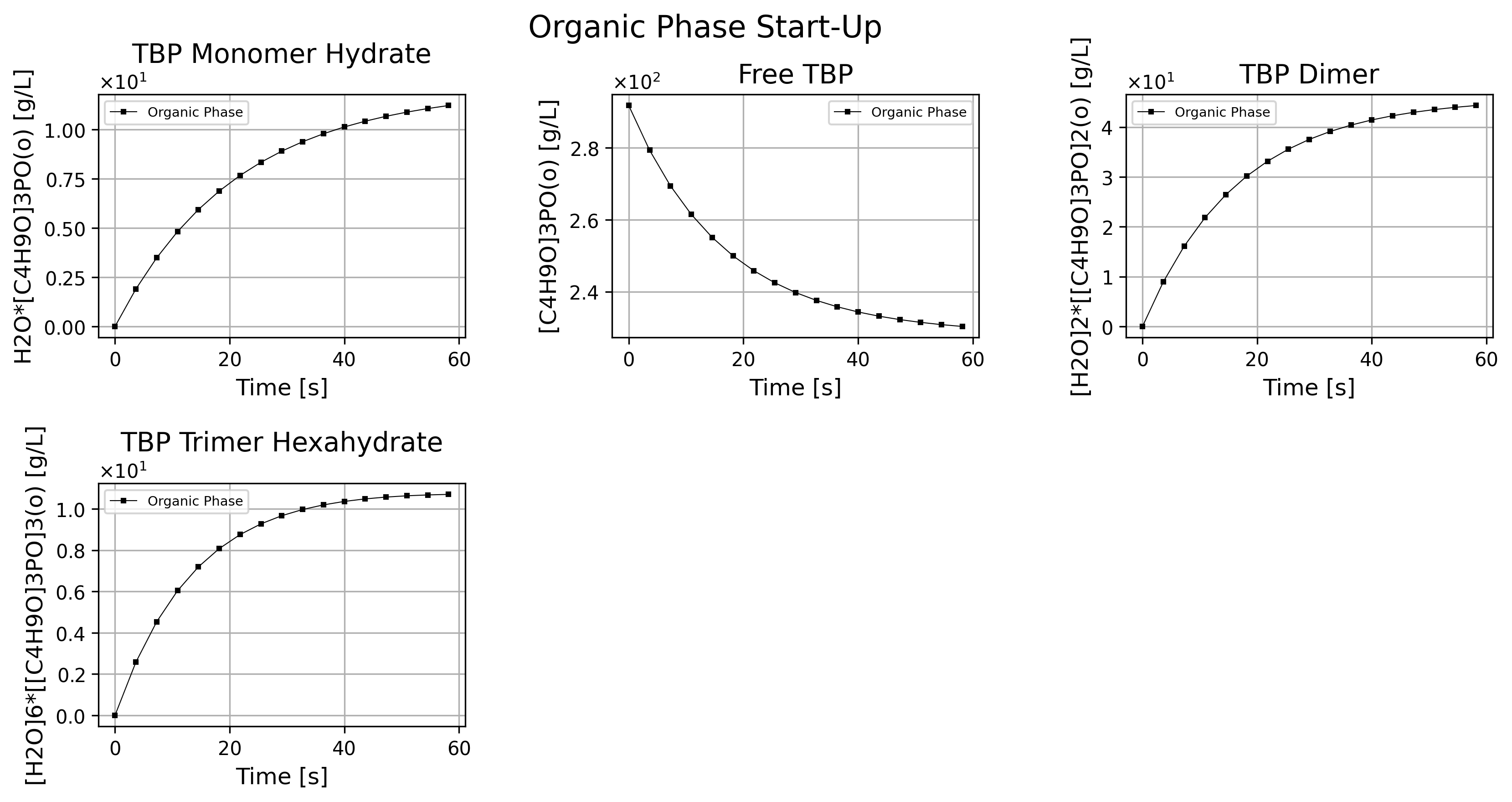
Figure 1: Organic phase species history dashboard at start-up.
'''Compute molar concentration of TBP species'''
import numpy as np

tbp_mass_cc_org_history = stg.organic_phase.get_column(tbp_org_name)
tbp_molar_cc_org_history = np.array(tbp_mass_cc_org_history)/tbp_org.molar_mass

tbp_monomer_mass_cc_org_history = stg.organic_phase.get_column(tbp_monomer_org_name)
tbp_monomer_molar_cc_org_history = np.array(tbp_monomer_mass_cc_org_history)/tbp_monomer_org.molar_mass

tbp_dimer_mass_cc_org_history = stg.organic_phase.get_column(tbp_dimer_org_name)
tbp_dimer_molar_cc_org_history = np.array(tbp_dimer_mass_cc_org_history)/tbp_dimer_org.molar_mass

tbp_trimer_hexahydrate_mass_cc_org_history = stg.organic_phase.get_column(tbp_trimer_hexahydrate_org_name)
tbp_trimer_hexahydrate_molar_cc_org_history = np.array(tbp_trimer_hexahydrate_mass_cc_org_history)/tbp_trimer_hexahydrate_org.molar_mass

time_stamps = np.array(stg.organic_phase.time_stamps)
n_startup = len(time_stamps)

tbl_count += 1
print(f'Table {tbl_count}: Molarity history of TBP in the organic phase at start-up.')
print('Time [min] | Free TBP [M] | TBP Monomer [M] | TBP Dimer [M] | TBP Trimer Hexahydrate [M] | balance |')
np.set_printoptions(precision=3, suppress=True, linewidth=100)
for t,a,b,c,d in zip(time_stamps[::5]/unit.min,
                 tbp_molar_cc_org_history[::5]/unit.molar,
                 tbp_monomer_molar_cc_org_history[::5]/unit.molar,
                 tbp_dimer_molar_cc_org_history[::5]/unit.molar,
                 tbp_trimer_hexahydrate_molar_cc_org_history[::5]/unit.molar):
    balance = a+b+2*c+3*d - tbp_mass_cc_org/tbp_org.molar_mass/unit.molar
    print('  %1.2e      %1.3f         %1.3e        %1.3e               %1.3e          %+1.3e'%(t, a, b, c, d, balance))
Table 1: Molarity history of TBP in the organic phase at start-up.
Time [min] | Free TBP [M] | TBP Monomer [M] | TBP Dimer [M] | TBP Trimer Hexahydrate [M] | balance |
  0.00e+00      1.096         0.000e+00        0.000e+00               0.000e+00          +0.000e+00
  3.03e-01      0.939         2.419e-02        5.303e-02               8.904e-03          -4.441e-16
  6.06e-01      0.885         3.443e-02        7.103e-02               1.124e-02          +0.000e+00
  9.09e-01      0.867         3.892e-02        7.730e-02               1.177e-02          +0.000e+00
'''Volume fraction of TBP at start-up'''
tbl_count += 1
print(f'Table {tbl_count}: Volume fractions of free and total TBP in the organic phase at start-up.')
print('Time [min] | Free TBP vol frac [%] | Total TBP vol frac [%] |')
np.set_printoptions(precision=3, suppress=True, linewidth=100)
total_tbp_molar_cc_org_history = tbp_molar_cc_org_history + tbp_monomer_molar_cc_org_history + \
                                 2*tbp_dimer_molar_cc_org_history + 3*tbp_trimer_hexahydrate_molar_cc_org_history
total_tbp_mass_cc_org_history = total_tbp_molar_cc_org_history * tbp_org.molar_mass
for t,a,b in zip(time_stamps[::5]/unit.min,
               np.array(tbp_mass_cc_org_history[::5])/rho_tbp*100, total_tbp_mass_cc_org_history[::5]/rho_tbp*100):
    print('  %1.2e         %1.3f                  %1.3f'%(t, a, b))
Table 2: Volume fractions of free and total TBP in the organic phase at start-up.
Time [min] | Free TBP vol frac [%] | Total TBP vol frac [%] |
  0.00e+00         30.000                  30.000
  3.03e-01         25.701                  30.000
  6.06e-01         24.244                  30.000
  9.09e-01         23.734                  30.000
'''Total water extracted'''
water_molar_cc_org_history = tbp_monomer_molar_cc_org_history \
                           + 2*tbp_dimer_molar_cc_org_history \
                           + 6*tbp_trimer_hexahydrate_molar_cc_org_history

water_mass_cc_org_history = water_molar_cc_org_history * h2o_aqu.molar_mass

tbl_count += 1
print(f'Table {tbl_count}: Mass concentration and molarity history of water in the organic phase at start-up.')
print('Time [s] |   [M]   |  [g/L]  |')
np.set_printoptions(precision=3, suppress=True, linewidth=100)
for a,b,c in zip(time_stamps[::5], water_molar_cc_org_history[::5]/unit.molar, water_mass_cc_org_history[::5]):
    print('%1.2e  %1.3e %1.3e'%(a, b, c))
Table 3: Mass concentration and molarity history of water in the organic phase at start-up.
Time [s] |   [M]   |  [g/L]  |
0.00e+00  0.000e+00 0.000e+00
1.82e+01  1.837e-01 3.309e+00
3.64e+01  2.439e-01 4.394e+00
5.45e+01  2.641e-01 4.758e+00
1.5.2. Aqueous Phase Results#
'''Plot aqueous phase'''
# TODO: time axis normalized by phase flow residence time.
stg.aqueous_phase.plot(title='Aqueous Phase Start-Up', legend='Aqueous Phase', nrows=2,ncols=3, show=True, figsize=[12,6])

fig_count += 1
print(f'Figure {fig_count}: Aqueous phase species history dashboard at start-up.')
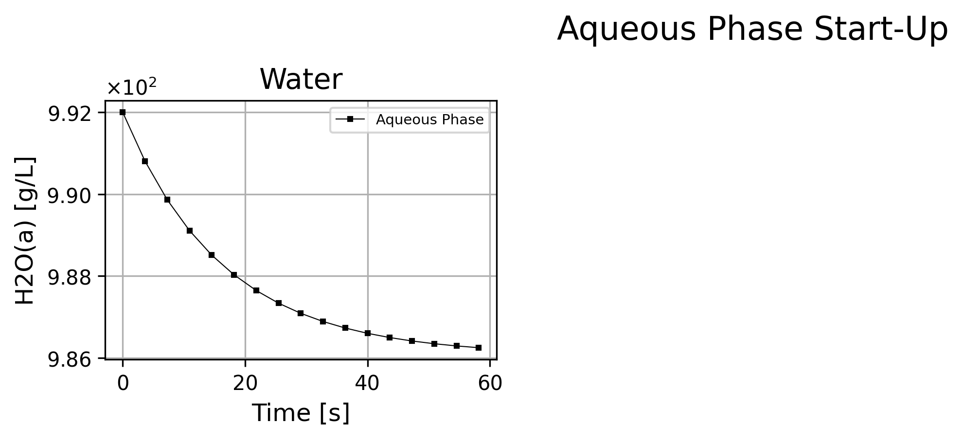
Figure 2: Aqueous phase species history dashboard at start-up.
1.5.3. Overall Stage Efficiency#
Stage efficiency measures how close to chemical equilibrium the system is as a whole. This is a direct result of the reaction relaxation time which is dependent on the mass transfer coefficients of the system. Much more needs to be investigated in this project with various degrees of theory but these results represent the beginning of a solid development.
'''Stage overall efficiency'''

quant = stg.efficiency_history(mean=True)
quant.plot(title='Stage Efficiency @ %2.1f C Start-Up'%unit.convert_temperature(stg_temperature,
           'K','C'), x_scaling=1/stg.flow_residence_time_avg, x_label=r'Time [$\bar{\tau}$]', y_label=quant.latex_name+
           ' ['+quant.unit+']', show=True, figsize=[10,3], error_data=True)

fig_count += 1
print(f'Figure {fig_count}: Stage efficiency history at start-up.')
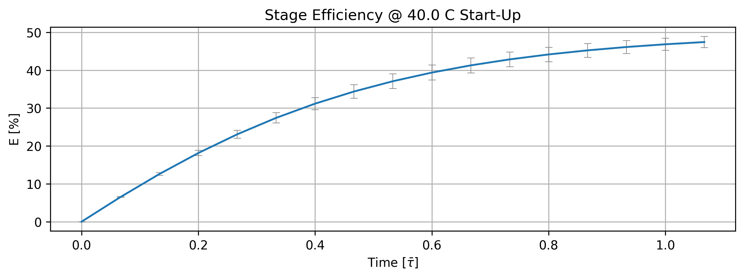
Figure 3: Stage efficiency history at start-up.
tbl_count += 1
print(f'Table {tbl_count}: Stage efficiency history at start-up.')
print('Time [min]  Stage. Eff.(+-std) [%]')
time_name = ''
import pandas as pd
df = (quant.value.apply(pd.Series).mul(1)
       .rename(index=lambda i: round(i/unit.min,2))
       .set_axis(['',''], axis=1).rename_axis(time_name)
       .round(3))
print(df.to_string(max_rows=20, min_rows=20))
Table 4: Stage efficiency history at start-up.
Time [min]  Stage. Eff.(+-std) [%]


0.00   0.000  0.000
0.06   6.507  0.111
0.12  12.589  0.377
0.18  18.131  0.711
0.24  23.077  1.052
0.30  27.417  1.359
0.36  31.171  1.611
0.42  34.380  1.797
0.48  37.096  1.919
0.55  39.378  1.982
0.61  41.282  1.994
0.67  42.862  1.965
0.73  44.167  1.904
0.79  45.242  1.820
0.85  46.125  1.720
0.91  46.848  1.610
0.97  47.439  1.495
'''Individual reaction efficiency'''
quant = stg.efficiency_history()
tbl_count += 1
print(f'Table {tbl_count}: Reaction efficiency history at start-up.')
print('Time [min]    Rxn Eff. [%]')

col_names = [f'r{i}' for i in range(len(stg.rxn_mech.reactions))]
time_name = ''
df = (quant.value.apply(pd.Series).mul(1)
       .rename(index=lambda i: round(i/unit.min,2))
       .set_axis(col_names, axis=1).rename_axis(time_name)
       .round(3))
print(df.to_string(max_rows=20, min_rows=20))
Table 5: Reaction efficiency history at start-up.
Time [min]    Rxn Eff. [%]
          r0      r1      r2

0.00   0.000   0.000   0.000
0.06   6.372   6.506   6.644
0.12  12.131  12.581  13.054
0.18  17.270  18.111  19.012
0.24  21.807  23.042  24.383
0.30  25.779  27.366  29.107
0.36  29.232  31.105  33.176
0.42  32.218  34.303  36.618
0.48  34.790  37.011  39.488
0.55  36.997  39.288  41.849
0.61  38.886  41.190  43.768
0.67  40.501  42.772  45.312
0.73  41.880  44.080  46.542
0.79  43.055  45.160  47.512
0.85  44.058  46.048  48.270
0.91  44.912  46.776  48.855
0.97  45.641  47.373  49.302
1.5.3.1. Total water extracted in equilibrium#
From reference: 1994 Naganawa and Tachimori Anal. Sci. 10 p 607
[H2O]_o,E = 0.4265 M
h2o_e_molar = water_molar_cc_org_history[-1]/unit.molar

print('Total H2O extracted [M] = %1.4f'%h2o_e_molar)
print('Error (compared to measurement) [%%] = %1.2f'%((h2o_e_molar-0.4265)/0.4265*100))
Total H2O extracted [M] = 0.2661
Error (compared to measurement) [%] = -37.60
1.5.4. Reaction Rate Density#
This quantity only makes sense per volume of the mixture.
'''Reaction rate density'''
import matplotlib.pyplot as plt

quant = stg.r_vec_history() # mole/m^3-s

quant.plot(title='Reaction Rate Density @ %2.1f C Start-Up'%unit.convert_temperature(stg_temperature,
           'K','C'), x_scaling=1/stg.flow_residence_time_avg, x_label=r'Time [$\bar{\tau}$]', y_label=quant.latex_name+
           ' ['+quant.unit+']', legend=stg.rxn_mech.reactions, show=True, figsize=[10,3], error_data=False)

fig_count += 1
print(f'Figure {fig_count}: Reaction rate density history at start-up.')
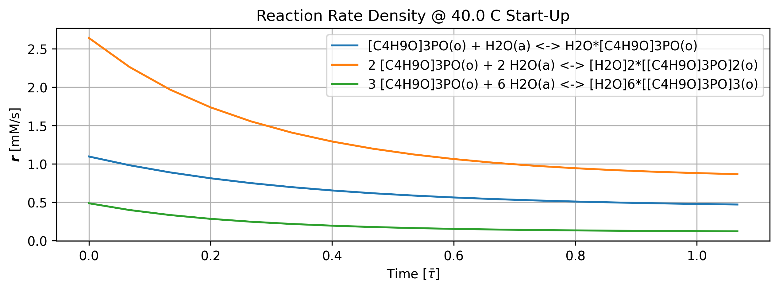
Figure 4: Reaction rate density history at start-up.
tbl_count += 1
print(f'Table {tbl_count}: Reaction rate density history at start-up.')
print('Time [min]      r [mM/s]')
import pandas as pd
col_names = [f'r{i}' for i in range(len(stg.rxn_mech.reactions))]
time_name = 't [min]'
df = (quant.value.apply(pd.Series).mul(1)
       .rename(index=lambda i: round(i/unit.min,2))
       .set_axis(col_names, axis=1).rename_axis(time_name)
       .round(4))
print(df.to_string(max_rows=20, min_rows=20))
Table 6: Reaction rate density history at start-up.
Time [min]      r [mM/s]
             r0      r1      r2
t [min]
0.00     1.0955  2.6403  0.4865
0.06     0.9820  2.2626  0.3985
0.12     0.8889  1.9681  0.3330
0.18     0.8122  1.7365  0.2836
0.24     0.7490  1.5533  0.2459
0.30     0.6966  1.4076  0.2169
0.36     0.6532  1.2912  0.1944
0.42     0.6171  1.1980  0.1770
0.48     0.5870  1.1231  0.1633
0.55     0.5620  1.0627  0.1527
0.61     0.5411  1.0141  0.1444
0.67     0.5235  0.9748  0.1378
0.73     0.5088  0.9430  0.1327
0.79     0.4965  0.9173  0.1287
0.85     0.4862  0.8964  0.1256
0.91     0.4774  0.8795  0.1232
0.97     0.4701  0.8658  0.1213
1.5.5. Species Generation Rate Density#
This quantity is on the basis of mixing volume so all species generation values can be compared.
'''Species generation rate density'''
import matplotlib.pyplot as plt

quant = stg.g_vec_history() # mole/m^3-s

quant.plot(title='Species Generation Rate Density @ %2.1f C Start-Up'%unit.convert_temperature(stg_temperature,
           'K','C'), x_scaling=1/stg.flow_residence_time_avg, x_label=r'Time [$\bar{\tau}$]', y_label=quant.latex_name+
           ' ['+quant.unit+']', legend=stg.rxn_mech.species_names, show=True, figsize=[10,3], error_data=False)

fig_count += 1
print(f'Figure {fig_count}: Species generation rate density history at start-up.')
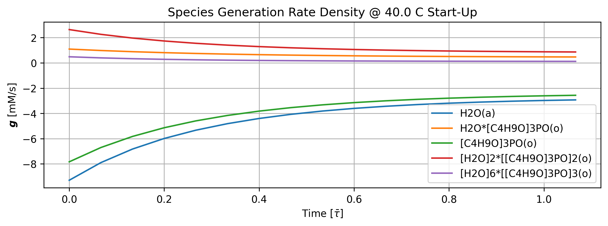
Figure 5: Species generation rate density history at start-up.
tbl_count += 1
print(f'Table {tbl_count}: Species generation rate density history at start-up.')
print('Time [min]        g [mM/s]')
import pandas as pd
col_names = [f'a{i}' for i in range(len(stg.rxn_mech.species_names))]
time_name = 't [min]'
df = (quant.value.apply(pd.Series).mul(1)
       .rename(index=lambda i: round(i/unit.min,2))
       .set_axis(col_names, axis=1).rename_axis(time_name)
       .round(4))
print(df.to_string(max_rows=20, min_rows=20))
Table 7: Species generation rate density history at start-up.
Time [min]        g [mM/s]
             a0      a1      a2      a3      a4
t [min]
0.00    -9.2949  1.0955 -7.8355  2.6403  0.4865
0.06    -7.8984  0.9820 -6.7028  2.2626  0.3985
0.12    -6.8231  0.8889 -5.8240  1.9681  0.3330
0.18    -5.9866  0.8122 -5.1359  1.7365  0.2836
0.24    -5.3306  0.7490 -4.5931  1.5533  0.2459
0.30    -4.8128  0.6966 -4.1623  1.4076  0.2169
0.36    -4.4020  0.6532 -3.8188  1.2912  0.1944
0.42    -4.0748  0.6171 -3.5439  1.1980  0.1770
0.48    -3.8132  0.5870 -3.3232  1.1231  0.1633
0.55    -3.6037  0.5620 -3.1456  1.0627  0.1527
0.61    -3.4354  0.5411 -3.0023  1.0141  0.1444
0.67    -3.3002  0.5235 -2.8866  0.9748  0.1378
0.73    -3.1912  0.5088 -2.7930  0.9430  0.1327
0.79    -3.1035  0.4965 -2.7173  0.9173  0.1287
0.85    -3.0327  0.4862 -2.6559  0.8964  0.1256
0.91    -2.9756  0.4774 -2.6061  0.8795  0.1232
0.97    -2.9296  0.4701 -2.5657  0.8658  0.1213
1.6. Steady-State Simulation#
Pick up from where it left from the past run() and continue to the fully developed state of 5 flow residence time. This demonstrates how to continue a simulation from where it was interrupted. Note that the state of the system is automatically used as the initial condition for the next run().
end_time += 4 * stg.flow_residence_time_avg
time_step = 4 * stg.flow_residence_time_avg / 10
show_time = (True, 10*time_step)

stg.time_step = time_step
stg.initial_time = stg.end_time
stg.end_time = end_time
stg.show_time = show_time
'''Run system in parallel'''
stg.monitor_mass_flowrates = False
stg.monitor_mass_conservation_residual = False
system.run()
system.close() # Shutdown Cortix
[13917] 2025-12-02 13:51:56,791 - cortix - INFO - Launching Module <solvex.stage.Stage object at 0x7f79dd878a50>
[13985] 2025-12-02 13:51:58,019 - cortix - INFO - Stg-1::run():time[m]=1.0
Total mass rate density (mixture volume) residual [g/L-s]= -9.02056e-17
total mass inflow rate [g/min]   = 6.710e+02
total mass outflow rate [g/min]  =  6.711e+02
	 net total mass flow rate [g/min] = 1.041e-13
[13985] 2025-12-02 13:51:58,127 - cortix - INFO - Stg-1::run():time[m]=4.6 (et[s]=0.1)
[13917] 2025-12-02 13:51:58,300 - cortix - INFO - run()::Elapsed wall clock time [s]: 6.49
[13917] 2025-12-02 13:51:58,301 - cortix - INFO - Closed Cortix object.
_____________________________________________________________________________
                           T E R M I N A T I N G
_____________________________________________________________________________
      ...                                        s       .     (TAAG Fraktur)
   xH88"`~ .x8X                                 :8      @88>
 :8888   .f"8888Hf        u.      .u    .      .88      %8P      uL   ..
:8888>  X8L  ^""`   ...ue888b   .d88B :@8c    :888ooo    .     .@88b  @88R
X8888  X888h        888R Y888r ="8888f8888r -*8888888  .@88u  ""Y888k/"*P
88888  !88888.      888R I888>   4888>"88"    8888    888E`    Y888L
88888   %88888      888R I888>   4888> "      8888      888E      8888
88888 `> `8888>     888R I888>   4888>        8888      888E      `888N
`8888L %  ?888   ! u8888cJ888   .d888L .+    .8888Lu=   888E   .u./"888&
 `8888  `-*""   /   "*888*P"    ^"8888*"     ^%888*     888&  d888" Y888*"
   "888.      :"      "Y"          "Y"         "Y"      R888" ` "Y   Y"
     `""***~"`                                           ""
                             https://cortix.org
_____________________________________________________________________________
[13917] 2025-12-02 13:51:58,301 - cortix - INFO - close()::Elapsed wall clock time [s]: 6.49
'''Recover stage'''
stg = system_net.modules[0]
1.6.1. Organic Phase Results#
'''Plot organic phase'''
# TODO: time axis normalized by phase flow residence time.
stg.organic_phase.plot(title='Organic Phase Steady-State', legend='Organic Phase', nrows=2,ncols=3, show=True, figsize=[12,6])

fig_count += 1
print(f'Figure {fig_count}: Organic phase species history dashboard at steady-state.')
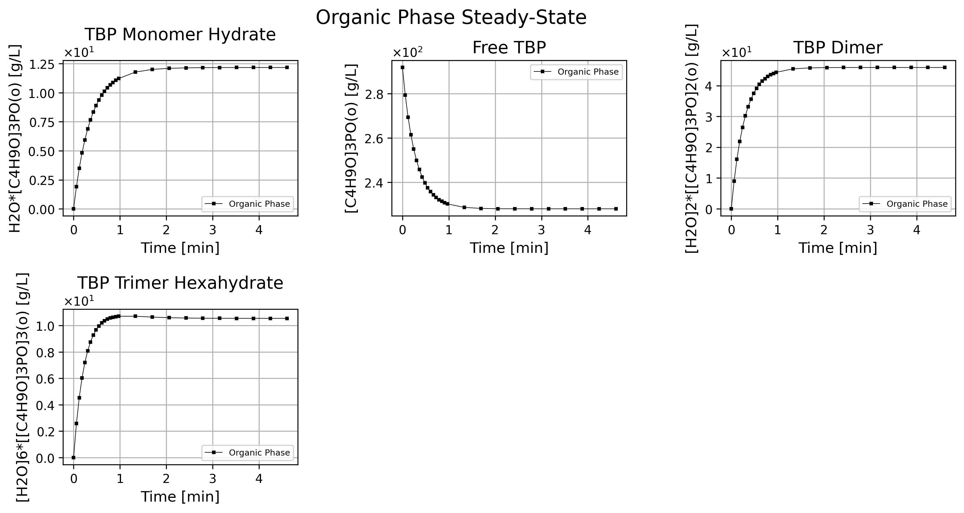
Figure 6: Organic phase species history dashboard at steady-state.
'''Compute molar concentration of TBP species'''
import numpy as np

tbp_mass_cc_org_history = stg.organic_phase.get_column(tbp_org_name)
tbp_molar_cc_org_history = np.array(tbp_mass_cc_org_history)/tbp_org.molar_mass

tbp_monomer_mass_cc_org_history = stg.organic_phase.get_column(tbp_monomer_org_name)
tbp_monomer_molar_cc_org_history = np.array(tbp_monomer_mass_cc_org_history)/tbp_monomer_org.molar_mass

tbp_dimer_mass_cc_org_history = stg.organic_phase.get_column(tbp_dimer_org_name)
tbp_dimer_molar_cc_org_history = np.array(tbp_dimer_mass_cc_org_history)/tbp_dimer_org.molar_mass

tbp_trimer_hexahydrate_mass_cc_org_history = stg.organic_phase.get_column(tbp_trimer_hexahydrate_org_name)
tbp_trimer_hexahydrate_molar_cc_org_history = np.array(tbp_trimer_hexahydrate_mass_cc_org_history)/tbp_trimer_hexahydrate_org.molar_mass

time_stamps = np.array(stg.organic_phase.time_stamps)

tbl_count += 1
print(f'Table {tbl_count}: Molarity history of TBP in the organic phase at steady-state.')
print('Time [min] | Free TBP [M] | TBP Monomer [M] | TBP Dimer [M] | TBP Trimer Hexahydrate [M] | balance |')
np.set_printoptions(precision=3, suppress=True, linewidth=100)
for t,a,b,c,d in zip(time_stamps[n_startup::5]/unit.min,
                 tbp_molar_cc_org_history[n_startup::5]/unit.molar,
                 tbp_monomer_molar_cc_org_history[n_startup::5]/unit.molar,
                 tbp_dimer_molar_cc_org_history[n_startup::5]/unit.molar,
                 tbp_trimer_hexahydrate_molar_cc_org_history[n_startup::5]/unit.molar):
    balance = a+b+2*c+3*d - tbp_mass_cc_org/tbp_org.molar_mass/unit.molar
    print('  %1.2e      %1.3f         %1.3e        %1.3e               %1.3e          %+1.3e'%(t, a, b, c, d, balance))
Table 8: Molarity history of TBP in the organic phase at steady-state.
Time [min] | Free TBP [M] | TBP Monomer [M] | TBP Dimer [M] | TBP Trimer Hexahydrate [M] | balance |
  1.33e+00      0.859         4.144e-02        7.991e-02               1.180e-02          +2.220e-16
  3.15e+00      0.856         4.280e-02        8.068e-02               1.163e-02          +0.000e+00
'''Volume fraction of TBP at start-up'''
tbl_count += 1
print(f'Table {tbl_count}: Volume fractions of free and total TBP in the organic phase at steady-state.')
print('Time [min] | Free TBP vol frac [%] | Total TBP vol frac [%] |')
np.set_printoptions(precision=3, suppress=True, linewidth=100)
total_tbp_molar_cc_org_history = tbp_molar_cc_org_history + tbp_monomer_molar_cc_org_history + \
                                 2*tbp_dimer_molar_cc_org_history + 3*tbp_trimer_hexahydrate_molar_cc_org_history
total_tbp_mass_cc_org_history = total_tbp_molar_cc_org_history * tbp_org.molar_mass
for t,a,b in zip(time_stamps[::5]/unit.min,
               np.array(tbp_mass_cc_org_history[::5])/rho_tbp*100, total_tbp_mass_cc_org_history[::5]/rho_tbp*100):
    print('  %1.2e         %1.3f                  %1.3f'%(t, a, b))
Table 9: Volume fractions of free and total TBP in the organic phase at steady-state.
Time [min] | Free TBP vol frac [%] | Total TBP vol frac [%] |
  0.00e+00         30.000                  30.000
  3.03e-01         25.701                  30.000
  6.06e-01         24.244                  30.000
  9.09e-01         23.734                  30.000
  2.42e+00         23.455                  30.000
  4.24e+00         23.453                  30.000
'''Total water extracted'''
water_molar_cc_org_history = tbp_monomer_molar_cc_org_history \
                           + 2*tbp_dimer_molar_cc_org_history \
                           + 6*tbp_trimer_hexahydrate_molar_cc_org_history

water_mass_cc_org_history = water_molar_cc_org_history * h2o_aqu.molar_mass

tbl_count += 1
print(f'Table {tbl_count}: Mass concentration and molarity history of water in the organic phase at steady-state.')
print('Time [s] |   [M]   |  [g/L]  |')
np.set_printoptions(precision=3, suppress=True, linewidth=100)
for a,b,c in zip(time_stamps[n_startup::5], water_molar_cc_org_history[n_startup::5]/unit.molar, water_mass_cc_org_history[n_startup::5]):
    print('%1.2e  %1.3e %1.3e'%(a, b, c))
Table 10: Mass concentration and molarity history of water in the organic phase at steady-state.
Time [s] |   [M]   |  [g/L]  |
8.00e+01  2.721e-01 4.901e+00
1.89e+02  2.739e-01 4.935e+00
1.6.2. Aqueous Phase Results#
'''Plot aqueous phase'''
# TODO: time axis normalized by phase flow residence time.
stg.aqueous_phase.plot(title='Aqueous Phase Steady-State', legend='Aqueous Phase', nrows=2,ncols=3, show=True, figsize=[12,6])

fig_count += 1
print(f'Figure {fig_count}: Aqueous phase species history dashboard at steady-state.')
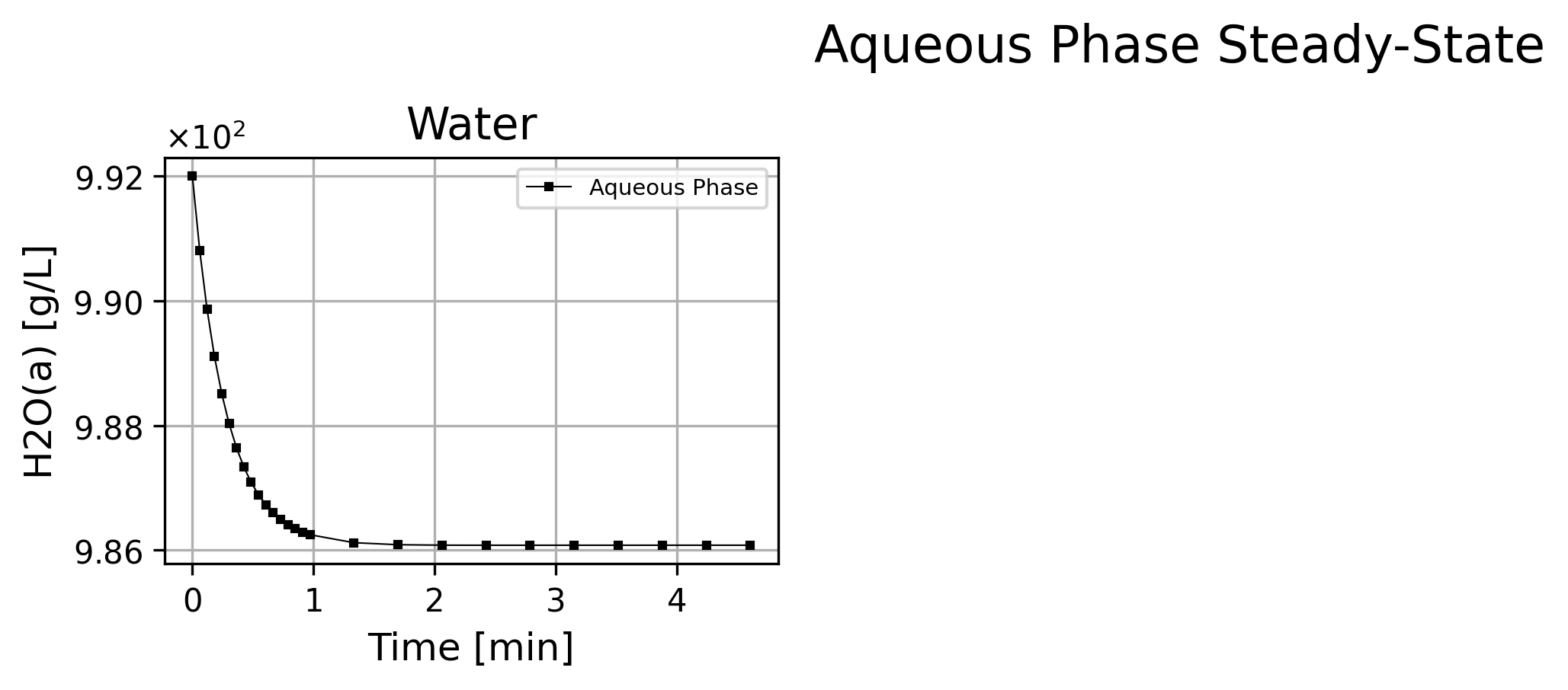
Figure 7: Aqueous phase species history dashboard at steady-state.
1.6.3. Overall Stage Efficiency#
'''Stage overall efficiency'''

quant = stg.efficiency_history(mean=True)
quant.plot(title='Stage Efficiency @ %2.1f C Steady-State'%unit.convert_temperature(stg_temperature,
           'K','C'), x_scaling=1/stg.flow_residence_time_avg, x_label=r'Time [$\bar{\tau}$]', y_label=quant.latex_name+
           ' ['+quant.unit+']', show=True, figsize=[10,3], error_data=True)

fig_count += 1
print(f'Figure {fig_count}: Stage efficiency history steady-state.')
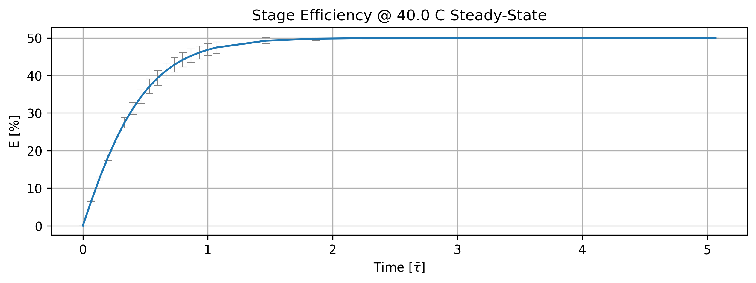
Figure 8: Stage efficiency history steady-state.
tbl_count += 1
print(f'Table {tbl_count}: Stage efficiency history at steady-state.')
print('Time [min]  Stage. Eff.(+-std) [%]')
time_name = ''
import pandas as pd
df = (quant.value.apply(pd.Series).mul(1)
       .rename(index=lambda i: round(i/unit.min,2))
       .set_axis(['',''], axis=1).rename_axis(time_name)
       .round(3))
print(df.to_string(max_rows=20, min_rows=20))
Table 11: Stage efficiency history at steady-state.
Time [min]  Stage. Eff.(+-std) [%]


0.00   0.000  0.000
0.06   6.507  0.111
0.12  12.589  0.377
0.18  18.131  0.711
0.24  23.077  1.052
0.30  27.417  1.359
0.36  31.171  1.611
0.42  34.380  1.797
0.48  37.096  1.919
0.55  39.378  1.982
...      ...    ...
1.33  49.276  0.855
1.70  49.800  0.437
2.06  49.947  0.211
2.42  49.987  0.099
2.79  49.997  0.046
3.15  50.000  0.021
3.52  50.000  0.010
3.88  50.000  0.004
4.24  50.000  0.002
4.61  50.000  0.001
'''Individual reaction efficiency'''
quant = stg.efficiency_history()
tbl_count += 1
print(f'Table {tbl_count}: Reaction efficiency history at steady-state.')
print('Time [min]    Rxn Eff. [%]')

col_names = [f'r{i}' for i in range(len(stg.rxn_mech.reactions))]
time_name = ''
df = (quant.value.apply(pd.Series).mul(1)
       .rename(index=lambda i: round(i/unit.min,2))
       .set_axis(col_names, axis=1).rename_axis(time_name)
       .round(3))
print(df.to_string(max_rows=20, min_rows=20))
Table 12: Reaction efficiency history at steady-state.
Time [min]    Rxn Eff. [%]
          r0      r1      r2

0.00   0.000   0.000   0.000
0.06   6.372   6.506   6.644
0.12  12.131  12.581  13.054
0.18  17.270  18.111  19.012
0.24  21.807  23.042  24.383
0.30  25.779  27.366  29.107
0.36  29.232  31.105  33.176
0.42  32.218  34.303  36.618
0.48  34.790  37.011  39.488
0.55  36.997  39.288  41.849
...      ...     ...     ...
1.33  48.246  49.241  50.339
1.70  49.274  49.784  50.343
2.06  49.692  49.940  50.210
2.42  49.867  49.984  50.110
2.79  49.942  49.996  50.054
3.15  49.974  49.999  50.026
3.52  49.989  50.000  50.012
3.88  49.995  50.000  50.005
4.24  49.998  50.000  50.002
4.61  49.999  50.000  50.001
1.6.3.1. Total water extracted in equilibrium#
From reference: 1994 Naganawa and Tachimori Anal. Sci. 10 p 607
[H2O]_o,E = 0.4265 M
Comparison to steady state:
h2o_e_molar = water_molar_cc_org_history[-1]/unit.molar

print('Total H2O extracted [M] = %1.4f'%h2o_e_molar)
print('Error (compared to measurement) [%%] = %1.2f'%((h2o_e_molar-0.4265)/0.4265*100))
Total H2O extracted [M] = 0.2739
Error (compared to measurement) [%] = -35.77
1.6.4. Reaction Rate Density#
This quantity only makes sense per volume of the mixture.
'''Reaction rate density'''
import matplotlib.pyplot as plt

quant = stg.r_vec_history()# mole/m^3-s

quant.plot(title='Reaction Rate Density @ %2.1f C Steady-State'%unit.convert_temperature(stg_temperature,
           'K','C'), x_scaling=1/stg.flow_residence_time_avg, x_label=r'Time [$\bar{\tau}$]', y_label=quant.latex_name+
           ' ['+quant.unit+']', legend=stg.rxn_mech.reactions, show=True, figsize=[10,3], error_data=False)

fig_count += 1
print(f'Figure {fig_count}: Reaction rate density history at steady-state.')
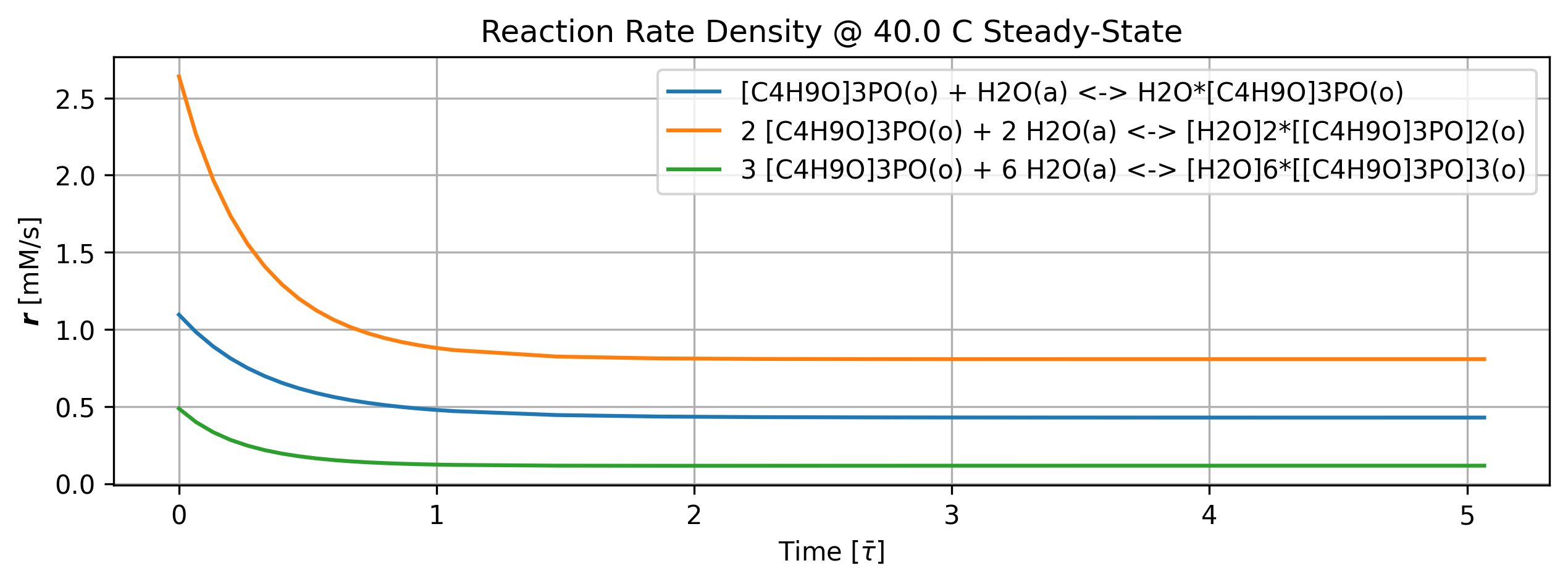
Figure 9: Reaction rate density history at steady-state.
tbl_count += 1
print(f'Table {tbl_count}: Reaction rate density history at steady-state.')
print('Time [min]      r [mM/s]')
import pandas as pd
col_names = [f'r{i}' for i in range(len(stg.rxn_mech.reactions))]
time_name = 't [min]'
df = (quant.value.apply(pd.Series).mul(1)
       .rename(index=lambda i: round(i/unit.min,2))
       .set_axis(col_names, axis=1).rename_axis(time_name)
       .round(4))
print(df.iloc[n_startup:].to_string(max_rows=20, min_rows=20))
Table 13: Reaction rate density history at steady-state.
Time [min]      r [mM/s]
             r0      r1      r2
t [min]
1.33     0.4445  0.8237  0.1164
1.70     0.4348  0.8117  0.1157
2.06     0.4310  0.8082  0.1158
2.42     0.4294  0.8072  0.1160
2.79     0.4287  0.8070  0.1161
3.15     0.4284  0.8069  0.1162
3.52     0.4283  0.8069  0.1162
3.88     0.4283  0.8069  0.1162
4.24     0.4282  0.8069  0.1162
4.61     0.4282  0.8069  0.1162
1.6.5. Species Generation Rate Density#
This quantity is on the basis of mixing volume so all species generation values can be compared.
'''Species generation rate density'''
import matplotlib.pyplot as plt

quant = stg.g_vec_history() # mole/m^3-s

quant.plot(title='Species Generation Rate Density @ %2.1f C Steady-State'%unit.convert_temperature(stg_temperature,
           'K','C'), x_scaling=1/stg.flow_residence_time_avg, x_label=r'Time [$\bar{\tau}$]', y_label=quant.latex_name+
           ' ['+quant.unit+']', legend=stg.rxn_mech.species_names, show=True, figsize=[10,3], error_data=False)

fig_count += 1
print(f'Figure {fig_count}: Species generation rate density history at steady-state.')
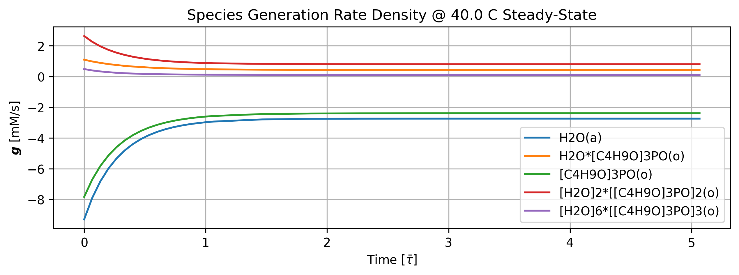
Figure 10: Species generation rate density history at steady-state.
tbl_count += 1
print(f'Table {tbl_count}: Species generation rate density history at steady-state.')
print('Time [min]        g [mM/s]')
import pandas as pd
col_names = [f'a{i}' for i in range(len(stg.rxn_mech.species_names))]
time_name = 't [min]'
df = (quant.value.apply(pd.Series).mul(1)
       .rename(index=lambda i: round(i/unit.min,2))
       .set_axis(col_names, axis=1).rename_axis(time_name)
       .round(4))
print(df.iloc[n_startup:].to_string(max_rows=20, min_rows=20))
Table 14: Species generation rate density history at steady-state.
Time [min]        g [mM/s]
             a0      a1      a2      a3      a4
t [min]
1.33    -2.7903  0.4445 -2.4411  0.8237  0.1164
1.70    -2.7523  0.4348 -2.4052  0.8117  0.1157
2.06    -2.7423  0.4310 -2.3948  0.8082  0.1158
2.42    -2.7398  0.4294 -2.3918  0.8072  0.1160
2.79    -2.7392  0.4287 -2.3909  0.8070  0.1161
3.15    -2.7392  0.4284 -2.3907  0.8069  0.1162
3.52    -2.7392  0.4283 -2.3906  0.8069  0.1162
3.88    -2.7392  0.4283 -2.3906  0.8069  0.1162
4.24    -2.7392  0.4282 -2.3906  0.8069  0.1162
4.61    -2.7392  0.4282 -2.3906  0.8069  0.1162
1.6.5.1. Species generation rate density at steady-state:#
g_vec = stg.g_vec()
columns = stg.rxn_mech.species_names
print('Generation sources [mM/s]')
print(pd.DataFrame([list(g_vec)], columns=columns).T
        .rename(columns={0:'g [mM/s]'}).to_string(float_format='{:.6f}'.format))
Generation sources [mM/s]
                         g [mM/s]
H2O(a)                  -2.739244
H2O*[C4H9O]3PO(o)        0.428233
[C4H9O]3PO(o)           -2.390595
[H2O]2*[[C4H9O]3PO]2(o)  0.806856
[H2O]6*[[C4H9O]3PO]3(o)  0.116216
1.7. Shut-down Simulation#
From steady-state, shutdown in two flow residence times.
end_time += 2 * stg.flow_residence_time_avg
time_step = 2 * stg.flow_residence_time_avg / 20
show_time = (True, 10*time_step)

stg.time_step = time_step
stg.initial_time = stg.end_time
stg.end_time = end_time
stg.show_time = show_time
'''Organic phase in the inflow'''
tbp_mass_cc_org = 0.0
stg.inflow_organic_phase.set_value(tbp_org_name, tbp_mass_cc_org)
'''Run system in parallel'''
stg.monitor_mass_flowrates = False
stg.monitor_mass_conservation_residual = False
system.run()
system.close() # Shutdown Cortix
[13917] 2025-12-02 13:52:00,870 - cortix - INFO - Launching Module <solvex.stage.Stage object at 0x7f79d9bf9090>
[14007] 2025-12-02 13:52:02,142 - cortix - INFO - Stg-1::run():time[m]=4.6
[14007] 2025-12-02 13:52:02,296 - cortix - INFO - Stg-1::run():time[m]=5.6
Total mass rate density (mixture volume) residual [g/L-s]= 1.73472e-18
total mass inflow rate [g/min]   = 4.960e+02
total mass outflow rate [g/min]  =  5.196e+02
	 net total mass flow rate [g/min] = 2.364e+01
[14007] 2025-12-02 13:52:02,423 - cortix - INFO - Stg-1::run():time[m]=6.4 (et[s]=0.3)
[13917] 2025-12-02 13:52:02,636 - cortix - INFO - run()::Elapsed wall clock time [s]: 10.83
[13917] 2025-12-02 13:52:02,637 - cortix - INFO - Closed Cortix object.
_____________________________________________________________________________
                           T E R M I N A T I N G
_____________________________________________________________________________
      ...                                        s       .     (TAAG Fraktur)
   xH88"`~ .x8X                                 :8      @88>
 :8888   .f"8888Hf        u.      .u    .      .88      %8P      uL   ..
:8888>  X8L  ^""`   ...ue888b   .d88B :@8c    :888ooo    .     .@88b  @88R
X8888  X888h        888R Y888r ="8888f8888r -*8888888  .@88u  ""Y888k/"*P
88888  !88888.      888R I888>   4888>"88"    8888    888E`    Y888L
88888   %88888      888R I888>   4888> "      8888      888E      8888
88888 `> `8888>     888R I888>   4888>        8888      888E      `888N
`8888L %  ?888   ! u8888cJ888   .d888L .+    .8888Lu=   888E   .u./"888&
 `8888  `-*""   /   "*888*P"    ^"8888*"     ^%888*     888&  d888" Y888*"
   "888.      :"      "Y"          "Y"         "Y"      R888" ` "Y   Y"
     `""***~"`                                           ""
                             https://cortix.org
_____________________________________________________________________________
[13917] 2025-12-02 13:52:02,638 - cortix - INFO - close()::Elapsed wall clock time [s]: 10.83
'''Recover stage'''
stg = system_net.modules[0]
1.7.1. Organic Phase Results#
'''Plot organic phase'''
# TODO: time axis normalized by phase flow residence time.
stg.organic_phase.plot(title='Organic Phase Shut-Down', legend='Organic Phase', nrows=2,ncols=3, show=True, figsize=[12,6])

fig_count += 1
print(f'Figure {fig_count}: Organic phase species history dashboard at shut-down.')
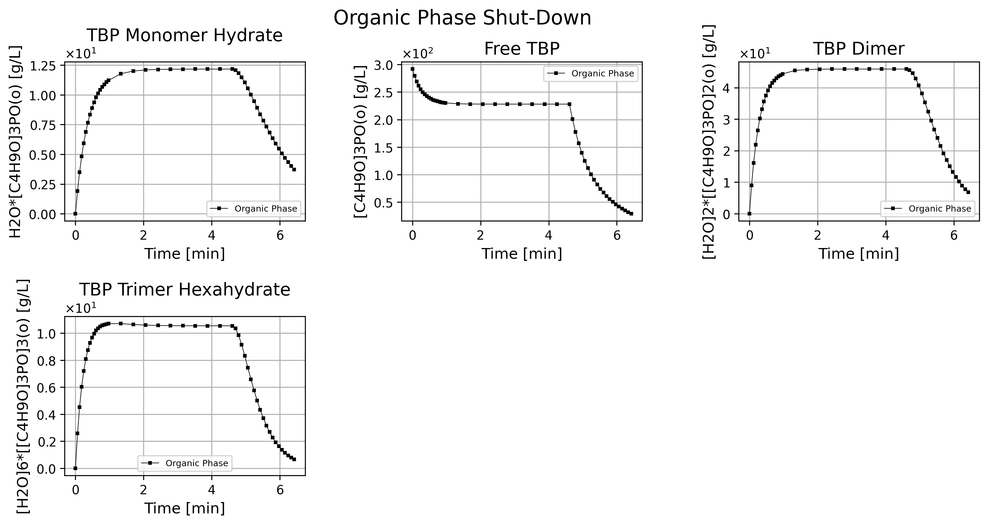
Figure 11: Organic phase species history dashboard at shut-down.
'''Compute molar concentration of TBP species'''
import numpy as np

tbp_mass_cc_org_history = stg.organic_phase.get_column(tbp_org_name)
tbp_molar_cc_org_history = np.array(tbp_mass_cc_org_history)/tbp_org.molar_mass

tbp_monomer_mass_cc_org_history = stg.organic_phase.get_column(tbp_monomer_org_name)
tbp_monomer_molar_cc_org_history = np.array(tbp_monomer_mass_cc_org_history)/tbp_monomer_org.molar_mass

tbp_dimer_mass_cc_org_history = stg.organic_phase.get_column(tbp_dimer_org_name)
tbp_dimer_molar_cc_org_history = np.array(tbp_dimer_mass_cc_org_history)/tbp_dimer_org.molar_mass

tbp_trimer_hexahydrate_mass_cc_org_history = stg.organic_phase.get_column(tbp_trimer_hexahydrate_org_name)
tbp_trimer_hexahydrate_molar_cc_org_history = np.array(tbp_trimer_hexahydrate_mass_cc_org_history)/tbp_trimer_hexahydrate_org.molar_mass

time_stamps = np.array(stg.organic_phase.time_stamps)

tbl_count += 1
print(f'Table {tbl_count}: Molarity history of TBP in the organic phase at shut-down.')
print('Time [min] | Free TBP [M] | TBP Monomer [M] | TBP Dimer [M] | TBP Trimer Hexahydrate [M] | balance |')
np.set_printoptions(precision=3, suppress=True, linewidth=100)
for t,a,b,c,d in zip(time_stamps[n_startup::5]/unit.min,
                 tbp_molar_cc_org_history[n_startup::5]/unit.molar,
                 tbp_monomer_molar_cc_org_history[n_startup::5]/unit.molar,
                 tbp_dimer_molar_cc_org_history[n_startup::5]/unit.molar,
                 tbp_trimer_hexahydrate_molar_cc_org_history[n_startup::5]/unit.molar):
    balance = a+b+2*c+3*d - tbp_mass_cc_org/tbp_org.molar_mass/unit.molar
    print('  %1.2e      %1.3f         %1.3e        %1.3e               %1.3e          %+1.3e'%(t, a, b, c, d, balance))
Table 15: Molarity history of TBP in the organic phase at shut-down.
Time [min] | Free TBP [M] | TBP Monomer [M] | TBP Dimer [M] | TBP Trimer Hexahydrate [M] | balance |
  1.33e+00      0.859         4.144e-02        7.991e-02               1.180e-02          +1.096e+00
  3.15e+00      0.856         4.280e-02        8.068e-02               1.163e-02          +1.096e+00
  4.70e+00      0.754         4.251e-02        8.015e-02               1.142e-02          +9.913e-01
  5.15e+00      0.420         3.526e-02        6.210e-02               7.264e-03          +6.012e-01
  5.61e+00      0.253         2.577e-02        3.783e-02               3.492e-03          +3.647e-01
  6.06e+00      0.158         1.787e-02        2.049e-02               1.506e-03          +2.212e-01
'''Volume fraction of TBP at start-up'''
tbl_count += 1
print(f'Table {tbl_count}: Volume fractions of free and total TBP in the organic phase at start-up.')
print('Time [min] | Free TBP vol frac [%] | Total TBP vol frac [%] |')
np.set_printoptions(precision=3, suppress=True, linewidth=100)
total_tbp_molar_cc_org_history = tbp_molar_cc_org_history + tbp_monomer_molar_cc_org_history + \
                                 2*tbp_dimer_molar_cc_org_history + 3*tbp_trimer_hexahydrate_molar_cc_org_history
total_tbp_mass_cc_org_history = total_tbp_molar_cc_org_history * tbp_org.molar_mass
for t,a,b in zip(time_stamps[::5]/unit.min,
               np.array(tbp_mass_cc_org_history[::5])/rho_tbp*100, total_tbp_mass_cc_org_history[::5]/rho_tbp*100):
    print('  %1.2e         %1.3f                  %1.3f'%(t, a, b))
Table 16: Volume fractions of free and total TBP in the organic phase at start-up.
Time [min] | Free TBP vol frac [%] | Total TBP vol frac [%] |
  0.00e+00         30.000                  30.000
  3.03e-01         25.701                  30.000
  6.06e-01         24.244                  30.000
  9.09e-01         23.734                  30.000
  2.42e+00         23.455                  30.000
  4.24e+00         23.453                  30.000
  4.97e+00         14.373                  20.110
  5.42e+00         8.425                  12.197
  5.88e+00         5.206                  7.398
  6.33e+00         3.277                  4.487
'''Total water extracted'''
water_molar_cc_org_history = tbp_monomer_molar_cc_org_history \
                           + 2*tbp_dimer_molar_cc_org_history \
                           + 6*tbp_trimer_hexahydrate_molar_cc_org_history

water_mass_cc_org_history = water_molar_cc_org_history * h2o_aqu.molar_mass

tbl_count += 1
print(f'Table {tbl_count}: Mass concentration and molarity history of water in the organic phase at shut-down.')
print('Time [s] |   [M]   |  [g/L]  |')
np.set_printoptions(precision=3, suppress=True, linewidth=100)
for a,b,c in zip(time_stamps[n_startup::5], water_molar_cc_org_history[n_startup::5]/unit.molar, water_mass_cc_org_history[n_startup::5]):
    print('%1.2e  %1.3e %1.3e'%(a, b, c))
Table 17: Mass concentration and molarity history of water in the organic phase at shut-down.
Time [s] |   [M]   |  [g/L]  |
8.00e+01  2.721e-01 4.901e+00
1.89e+02  2.739e-01 4.935e+00
2.82e+02  2.713e-01 4.888e+00
3.09e+02  2.030e-01 3.658e+00
3.36e+02  1.224e-01 2.205e+00
3.64e+02  6.788e-02 1.223e+00
1.7.2. Aqueous Phase Results#
'''Plot aqueous phase'''
# TODO: time axis normalized by phase flow residence time.
stg.aqueous_phase.plot(title='Aqueous Phase Shut-Down', legend='Aqueous Phase', nrows=2,ncols=3, show=True, figsize=[12,6])

fig_count += 1
print(f'Figure {fig_count}: Aqueous phase species history dashboard at shut-down.')
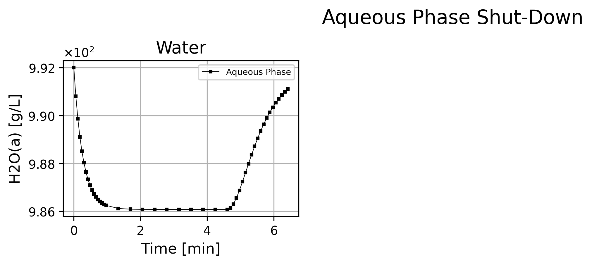
Figure 12: Aqueous phase species history dashboard at shut-down.
1.7.3. Reaction Rate Density#
This quantity only makes sense per volume of the mixture.
'''Reaction rate density'''
import matplotlib.pyplot as plt

quant = stg.r_vec_history()
quant.plot(title='Reaction Rate Density @ %2.1f C Shut-Down'%unit.convert_temperature(stg_temperature,
           'K','C'), x_scaling=1/stg.flow_residence_time_avg, x_label=r'Time [$\bar{\tau}$]', y_label=quant.latex_name+
           ' ['+quant.unit+']', legend=stg.rxn_mech.reactions, show=True, figsize=[10,3], error_data=False)

fig_count += 1
print(f'Figure {fig_count}: Reaction rate density history at shut-down.')
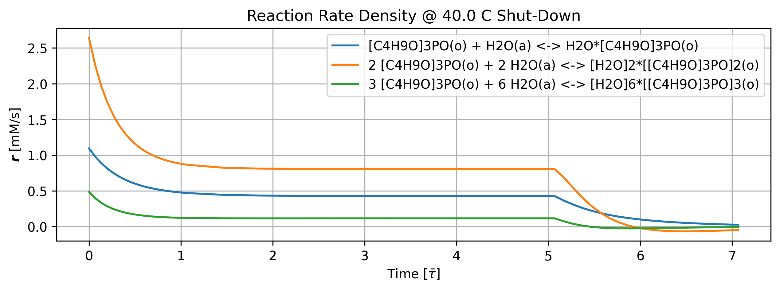
Figure 13: Reaction rate density history at shut-down.
1.7.4. Species Generation Rate Density#
This quantity is on the basis of mixing volume so all species generation values can be compared.
'''Species generation rate density'''
import matplotlib.pyplot as plt

quant = stg.g_vec_history()
quant.plot(title='Species Generation Rate Density @ %2.1f C Shut-Down'%unit.convert_temperature(stg_temperature,
           'K','C'), x_scaling=1/stg.flow_residence_time_avg, x_label=r'Time [$\bar{\tau}$]', y_label=quant.latex_name+
           ' ['+quant.unit+']', legend=stg.rxn_mech.species_names, show=True, figsize=[10,3], error_data=False)

fig_count += 1
print(f'Figure {fig_count}: Species generation rate density history at shut-down.')
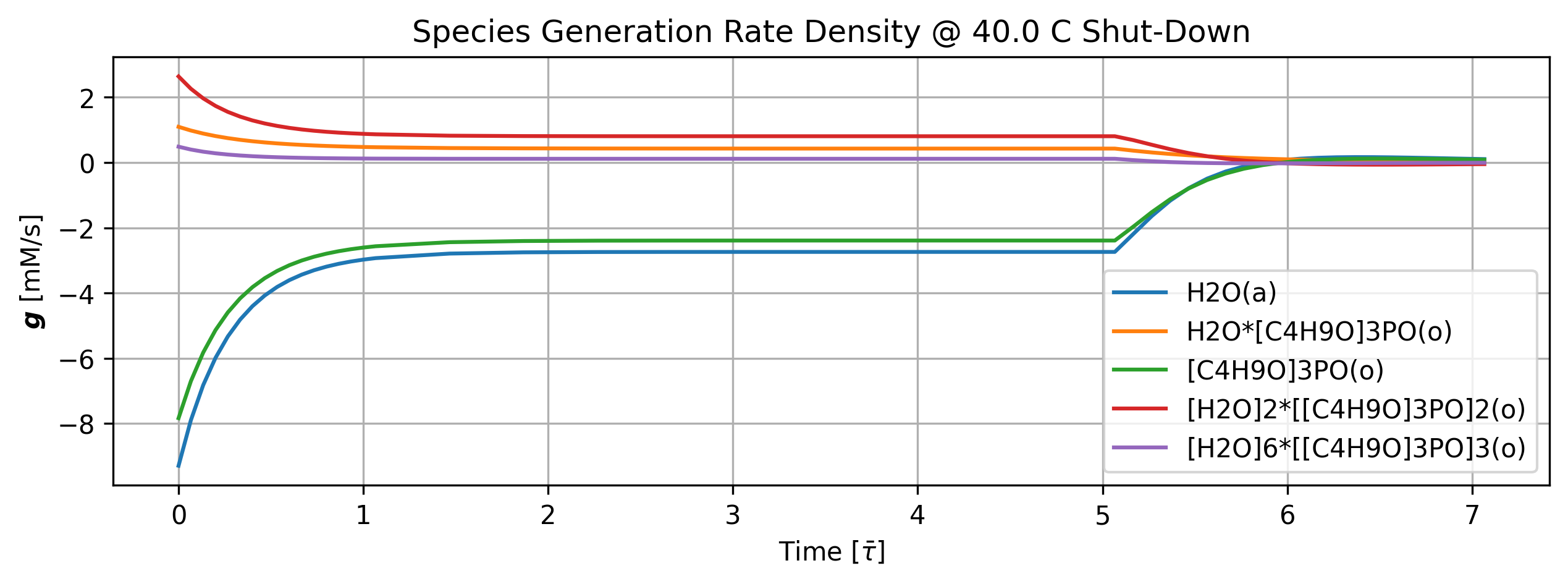
Figure 14: Species generation rate density history at shut-down.
1.8. References#
[1] V. F. de Almeida, Cortix, Network Dynamics Simulation, Cortix Tech, Lowell, MA.