Single-Stage Solvex Development Cortix Tech 30Sep2025

1. Use-Case 02.1: TBP-Diluent-H\(_2\)O-Air Mixing Parameter Study

Developer: Valmor F. de Almeida, PhD

Cortix Tech, Lowell, MA 01854, USA

Revision date: 19Nov25

Early stage of parametric study simulation using Cortix. The goal here is to provide a mininum framework to help the testing of fixed-parameter simulations.

1.1. Objectives

• Develop a usecase scenario for water extraction by TBP with a vapor phase parametric study.

• Test implementation and present results.

'''AI assistance options'''
# Set all to False if you do not have access to OpenAI API and/or AI codes below
cortix_ai = True

'''Generate proprietary knowledge database?'''
db_save = False # set this to false if going public (online) with this notebook

'''Other helpers'''
fig_count = 0
tbl_count = 0
markdown_display = True # if False code cell output is type: stream, else: markdown. Use True for in-house conversion to .md

1.2. Mass Transfer and Inflow Relative Humidity Variation

The entire system is prepared as a batch job.

'''Read batch run file'''
from run_tbp_h2o_air import main as run

if cortix_ai:
    from cortix import CortixAI
    cortix_ai = CortixAI(llm_model='gpt-5-mini', llm_cleverness=0.8)
    cortix_ai.markdown_header_level = 'h3'

if cortix_ai:
    cortix_ai.explain(markdown_display=markdown_display, save_supporting_info=db_save)

Cortix AI assistant: working on explanation...

Overview

This snippet is a small Python module that imports a function, conditionally constructs a CortixAI object, configures it, and then calls a method on that object. It relies on several names (cortix_ai, markdown_display, db_save) that must exist in the surrounding runtime.

Line-by-line explanation

• The first line is a module-level docstring: ‘Read batch run file’.

• from run_tbp_h2o_air import main as run

  • Imports the name main from the module run_tbp_h2o_air and binds it locally as run.

• if cortix_ai:

  • Tests the truthiness of the name cortix_ai at runtime. If that name is not defined, evaluating this condition raises a NameError; if defined and truthy, the block executes.

  • from cortix import CortixAI

    • Imports the CortixAI class (or factory) from the cortix package, at the moment the condition is true.

  • cortix_ai = CortixAI(llm_model=’gpt-5-mini’, llm_cleverness=0.8)

    • Creates an instance of CortixAI with the keyword arguments llm_model set to ‘gpt-5-mini’ and llm_cleverness set to 0.8, then assigns that instance to the name cortix_ai, overwriting the previous value of cortix_ai.

  • cortix_ai.markdown_header_level = ‘h3’

    • Sets an attribute markdown_header_level on the newly created CortixAI instance to the string ‘h3’.

• if cortix_ai:

  • Re-evaluates the truthiness of cortix_ai; since cortix_ai was just assigned to an instance in the prior block (when that block ran), this will typically be true and the following call will execute.

  • cortix_ai.explain(markdown_display=markdown_display, save_supporting_info=db_save)

    • Invokes the explain method on the cortix_ai instance, passing two keyword arguments: markdown_display and save_supporting_info whose values are taken from the names markdown_display and db_save in the current namespace.

Runtime dependencies and behavior

• The snippet assumes these names exist in the runtime before execution:

  • cortix_ai (checked and later overwritten)

  • markdown_display (passed to explain)

  • db_save (passed as save_supporting_info)

• The import of CortixAI happens only if the first if cortix_ai condition is true; that import is not executed at module import time unless the condition is met at runtime.

• The code rebinds cortix_ai inside the first conditional, so the value checked by the second if cortix_ai may be the same object created in the first block.

• The alias run refers to run_tbp_h2o_air.main and is available for use elsewhere in the module after this snippet.

CortixAI configuration present in the snippet

• llm_model=’gpt-5-mini’ — selects the language model identifier passed to CortixAI.

• llm_cleverness=0.8 — sets a numeric parameter named llm_cleverness on instantiation.

• markdown_header_level = ‘h3’ — sets the instance attribute that controls the header level for Markdown output.

Contextual notes

• This code pattern is typical where a runtime flag or pre-existing object determines whether to construct and use an AI helper object and to emit Markdown-formatted output in an interactive environment (for example, a Jupyter notebook).

AI Parameters:
+ LLM model (OpenAI) = gpt-5-mini
+ LLM cleverness     = 1.0
+ Total # of tokens  = 3509

'''Prepare Params Dictionary'''
params = dict()
params['make-plots'] = False
params['verbose'] = False
params['loglevel'] = 'error'

Here the base relaxation time of all reactions is progressively increased and all stage data saved for future efficiency analysis.

'''Vary Parameter of Study'''
stages = list()

rxn_tau_multipliers = (1.0, 1.2, 0.7, 0.5, 0.8, 0.9) # flow residence time multipliers
param_tau_factors = [0.1, 0.5, 1.0, 1.5] # parameter variation
#param_tau_factors = [1, 1, 1, 1]

inflow_relative_humidity = 25
param_inflow_rh_factors = [0.1, 0.5, 1.0, 1.5] # parameter variation
#param_inflow_rh_factors = [0.2, 1, 1.7, 3.9]

assert len(param_tau_factors) == len(param_inflow_rh_factors)
for param_tau_factor, param_inflow_rh_factor in zip(param_tau_factors, param_inflow_rh_factors):
    
    params['tau-factor-0'] = rxn_tau_multipliers[0] * param_tau_factor
    params['tau-factor-1'] = rxn_tau_multipliers[1] * param_tau_factor
    params['tau-factor-2'] = rxn_tau_multipliers[2] * param_tau_factor
    print('tau-factor ', param_tau_factor)

    params['inflow-relative-humidity'] = param_inflow_rh_factor * inflow_relative_humidity
    print('inflow-relative-humidity ', params['inflow-relative-humidity'])
    
    stg = run(params)
    
    stages.append(stg)

if cortix_ai:
    cortix_ai.explain(markdown_display=markdown_display, save_supporting_info=db_save)

tau-factor  0.1
inflow-relative-humidity  2.5
Total mass rate density (mixture volume) residual [g/L-s]= -5.71713e-17
total mass inflow rate [g/min]   = 7.471e+02
total mass outflow rate [g/min]  =  7.471e+02
	 net total mass flow rate [g/min] = -3.770e-02
tau-factor  0.5
inflow-relative-humidity  12.5
Total mass rate density (mixture volume) residual [g/L-s]= -1.08169e-16
total mass inflow rate [g/min]   = 7.471e+02
total mass outflow rate [g/min]  =  7.471e+02
	 net total mass flow rate [g/min] = -3.769e-02
tau-factor  1.0
inflow-relative-humidity  25.0
Total mass rate density (mixture volume) residual [g/L-s]= -3.44709e-17
total mass inflow rate [g/min]   = 7.471e+02
total mass outflow rate [g/min]  =  7.471e+02
	 net total mass flow rate [g/min] = -3.767e-02
tau-factor  1.5
inflow-relative-humidity  37.5
Total mass rate density (mixture volume) residual [g/L-s]= -3.07371e-17
total mass inflow rate [g/min]   = 7.471e+02
total mass outflow rate [g/min]  =  7.471e+02
	 net total mass flow rate [g/min] = -3.649e-02
Cortix AI assistant: working on explanation...

Overview

• This snippet runs a small parameter sweep: it varies two linked parameters (a set of “tau” multipliers and an inflow relative-humidity factor) across matching factor vectors, runs a simulation/function for each combination, and collects the returned stage results in a list named stages.

Key variables and their roles

• stages

  • An initially empty list that collects the return value from each call to run(params).

• rxn_tau_multipliers

  • A tuple of base multipliers for reaction/flow residence time (comment: “flow residence time multipliers”). The code uses indices 0, 1 and 2 of this tuple.

• param_tau_factors

  • A list of scalar factors by which the rxn_tau_multipliers are scaled for each sweep iteration.

• inflow_relative_humidity

  • A base numeric value (25) representing the reference inflow relative humidity.

• param_inflow_rh_factors

  • A list of scalar factors applied to inflow_relative_humidity for each sweep iteration.

• params

  • An assumed pre-existing mapping (e.g., dict) that is being updated in-place inside the loop with keys ‘tau-factor-0’, ‘tau-factor-1’, ‘tau-factor-2’, and ‘inflow-relative-humidity’.

• run(params)

  • A call to an external function (assumed to perform the simulation or computation) whose return value is appended to stages.

• cortix_ai (and its method call)

  • A variable checked after the sweep; if truthy, cortix_ai.explain(…) is invoked. (No explanation of that method’s behavior is given here.)

Control flow and computations

• The assertion assert len(param_tau_factors) == len(param_inflow_rh_factors) enforces that the two factor lists have the same length; otherwise the script will raise an AssertionError and stop.

• The for loop iterates in parallel over param_tau_factors and param_inflow_rh_factors using zip; with the provided lists the loop runs four iterations (one per factor pair).

• Inside each iteration:

  • The code sets three params entries:

    • params[‘tau-factor-0’] = rxn_tau_multipliers[0] * param_tau_factor

    • params[‘tau-factor-1’] = rxn_tau_multipliers[1] * param_tau_factor

    • params[‘tau-factor-2’] = rxn_tau_multipliers[2] * param_tau_factor

  • A print statement outputs the current param_tau_factor.

  • The inflow-relative-humidity parameter is updated as params[‘inflow-relative-humidity’] = param_inflow_rh_factor * inflow_relative_humidity and printed.

  • run(params) is invoked; its return value is stored in stg and appended to stages.

• After the loop, if cortix_ai is truthy, cortix_ai.explain(markdown_display=markdown_display, save_supporting_info=db_save) is called.

Concrete numeric example (first iteration)

• With the first pair param_tau_factor = 0.1 and param_inflow_rh_factor = 0.1:

  • params[‘tau-factor-0’] = 1.0 * 0.1 = 0.1

  • params[‘tau-factor-1’] = 1.2 * 0.1 = 0.12

  • params[‘tau-factor-2’] = 0.7 * 0.1 = 0.07

  • params[‘inflow-relative-humidity’] = 0.1 * 25 = 2.5

  • Then run(params) is executed and its result appended to stages.

Additional notes and observable behaviors

• Only the first three entries of rxn_tau_multipliers are used; the tuple contains six values but indices 3–5 are not referenced by this code.

• The commented-out alternate lists are inactive and have no effect.

• The printed lines provide runtime visibility of each iteration’s param_tau_factor and the computed inflow-relative-humidity value.

• stages ends up with one element per iteration (four elements for the provided factor lists), each element being whatever run(params) returned.

AI Parameters:
+ LLM model (OpenAI) = gpt-5-mini
+ LLM cleverness     = 1.0
+ Total # of tokens  = 4061

1.2.1. Overall Stage Efficiency

Parameter variation impact on stage efficiency.

'''Stage overall efficiency'''
from cortix import Units as unit
import matplotlib.pyplot as plt

efficiencies = list()

for stg in stages:
    efficiencies.append(stg.efficiency_history(mean=True))

for eff, tau, rh in zip(efficiencies, param_tau_factors, param_inflow_rh_factors):
    quant = eff
    # Edit quant for AI use below
    quant.name += f"""; @ parameter tau factor = {tau} and parameter relative humidity {rh}"""
    quant.value.name = quant.name
    quant.plot(title=r'Stage Efficiency w/ $\tau_{\mathrm{f}}$ = %2.1f; rh$_{\mathrm{f}}$ = %2.1f'%(tau,rh), x_scaling=1/unit.min, x_label='Time [min]', y_label=quant.latex_name+
               ' ['+quant.unit+']', show=True, figsize=[10,3], error_data=True, error_fill=False)
if cortix_ai: 
    cortix_ai.explain(markdown_display=markdown_display, save_supporting_info=db_save)

fig_count += 1
print(f'Figure {fig_count}: Stage efficiency variation with parameters.')

Cortix AI assistant: working on explanation...

Overview

This snippet collects stage efficiencies, annotates each efficiency object with the corresponding parameter values, and produces a plot per paired parameter set. It also conditionally invokes a Cortix AI helper and updates a figure counter.

• The script imports Units from cortix as unit and matplotlib.pyplot as plt, then declares an empty list efficiencies.

• It builds efficiencies by iterating for stg in stages: and appending stg.efficiency_history(mean=True). Each appended item is expected to be an object (hereafter “quant”) representing a time series or quantity with attributes and a plot method.

• The for eff, tau, rh in zip(efficiencies, param_tau_factors, param_inflow_rh_factors): loop iterates over tuples formed by zipping the three iterables; iteration stops when the shortest iterable is exhausted.

• Inside the loop:

  • quant = eff binds the current efficiency object to the name quant.

  • quant.name += f"""; @ parameter tau factor = {tau} and parameter relative humidity {rh}""" appends a semicolon-delimited annotation containing the numeric tau and rh to the existing quant.name string.

  • quant.value.name = quant.name assigns the same annotated name to an inner attribute quant.value.name.

  • quant.plot(...) is called with these keyword arguments:

    • title built with a raw string that embeds tau and rh using the %2.1f format specifiers and includes LaTeX-style fragments inside the raw string.

    • x_scaling=1/unit.min — an x-axis scaling factor that converts the internal x units to minutes by multiplying x-data by this factor (since unit.min denotes one minute in the cortix Units system).

    • x_label='Time [min]'

    • y_label=quant.latex_name + ' [' + quant.unit + ']' — the y-axis label concatenates a LaTeX-ready name and the unit in brackets.

    • show=True — request to display the plot immediately.

    • figsize=[10,3] — figure dimensions in inches (width, height).

    • error_data=True and error_fill=False — plotting options controlling how uncertainty/error is rendered.

  • The call to quant.plot is a method on the quant object and is responsible for creating the matplotlib figure (and potentially other side effects like logging or storing the figure), based on the provided metadata and data.

• After the plotting loop, the code conditionally executes if cortix_ai: cortix_ai.explain(markdown_display=markdown_display, save_supporting_info=db_save). This calls the explain method on cortix_ai when cortix_ai is truthy, passing two named arguments; the contents or behavior of explain are not described here.

• Finally, fig_count += 1 increments a figure counter, and print(f'Figure {fig_count}: Stage efficiency variation with parameters.') emits a short status message referencing the new figure count.

Key variables and expected types

• stages: an iterable of stage objects; each stage must provide an efficiency_history(mean=True) method that returns a quant-like object.

• efficiencies: Python list of the returned quant objects.

• param_tau_factors, param_inflow_rh_factors: iterables (lists/tuples/arrays) of numeric parameter values; zipped with efficiencies for one-to-one plotting.

• quant (each item in efficiencies):

  • attributes used: name (string), value (object with .name), latex_name (string), unit (string),

  • method used: .plot(...) taking plotting metadata and options.

• unit.min: a numeric value from the cortix Units system representing one minute; used to compute x_scaling = 1 / unit.min.

• cortix_ai, markdown_display, db_save: variables referenced for the conditional explain call; presence and truthiness control that invocation.

• fig_count: an integer counter incremented after plotting.

Side effects and outputs

• The code mutates each quant by appending parameter information to quant.name and copying that to quant.value.name.

• It produces one plot per zipped tuple; plots are created via quant.plot with show=True, so they are displayed immediately (typical effect in a Jupyter session is an inline figure).

• The zip(...) means if the three sequences differ in length, only the length of the shortest sequence will be processed.

• If cortix_ai is truthy, a method call with markdown_display and save_supporting_info=db_save is made on that object.

• fig_count is incremented and a print statement logs the figure index and a short description.

AI Parameters:
+ LLM model (OpenAI) = gpt-5-mini
+ LLM cleverness     = 1.0
+ Total # of tokens  = 4117
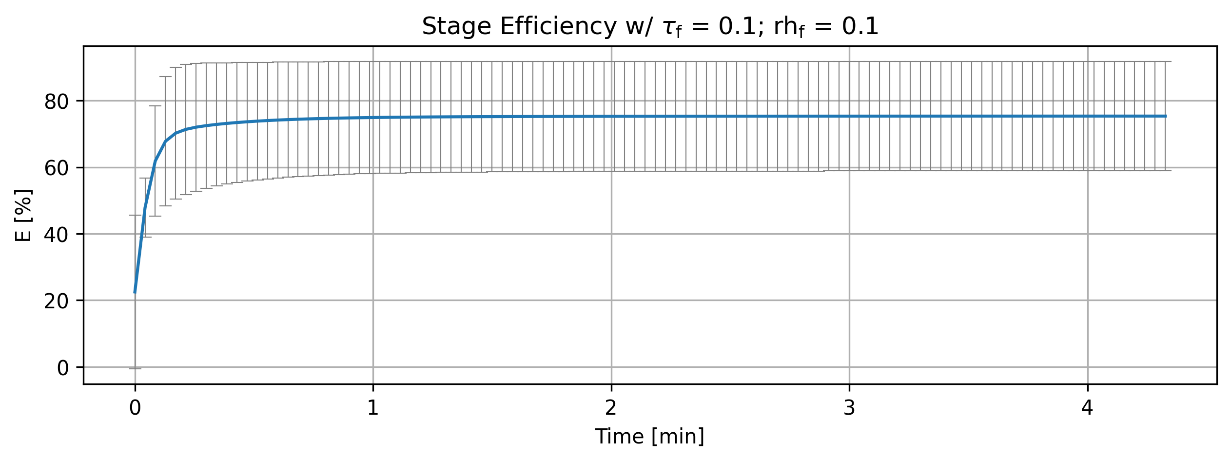
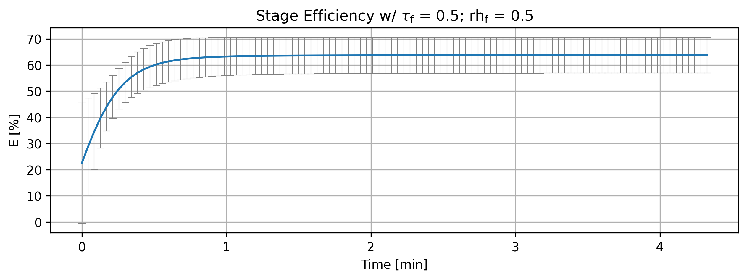
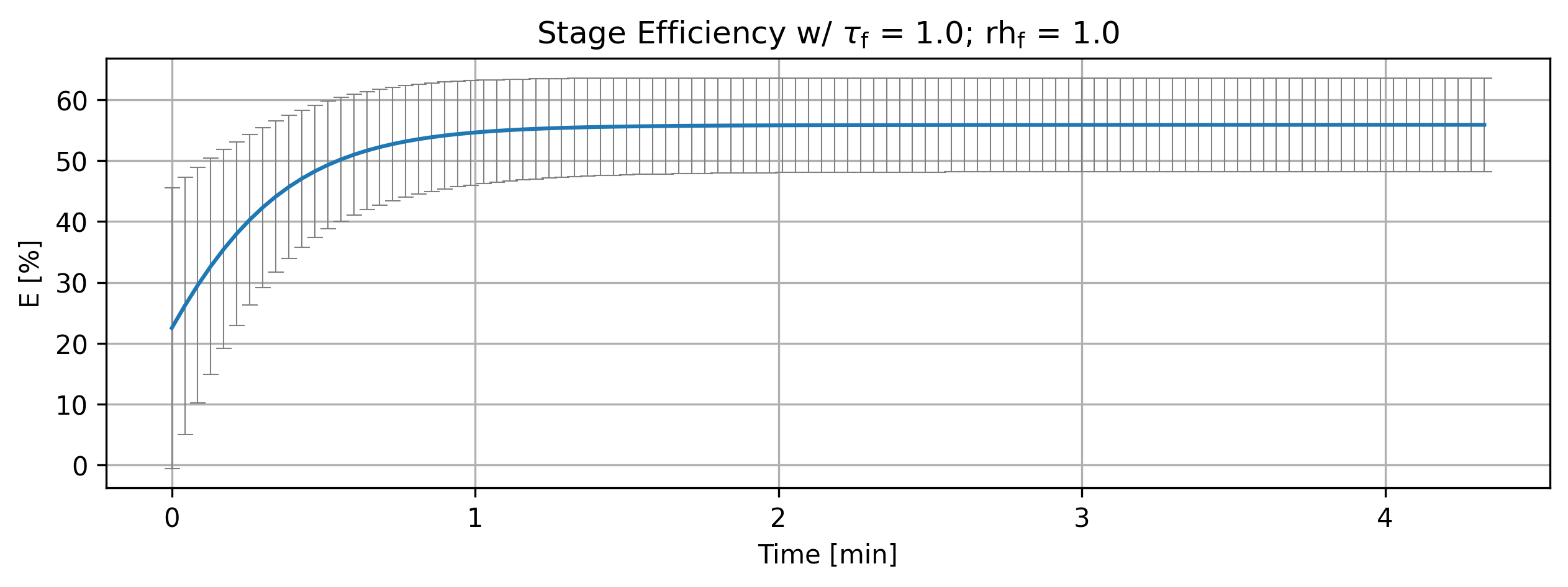
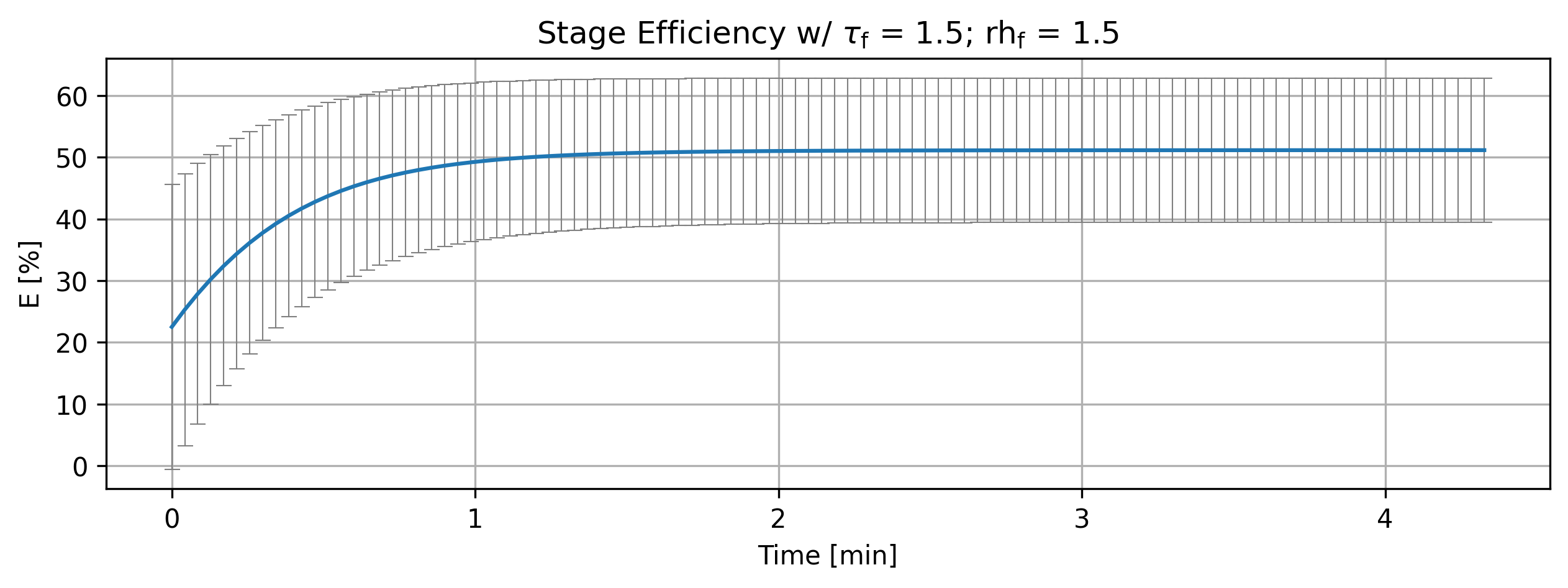
Figure 1: Stage efficiency variation with parameters.

1.2.2. Analysis

LLM analysis.

'''Analyze efficiencies'''
if cortix_ai: 
    cortix_ai.explain(quant=efficiencies, markdown_header_level='<h4>', markdown_display=markdown_display, save_supporting_info=db_save)

Cortix AI assistant: working on explanation...

Overview

• Data: time histories (0 → 246.765 s) of Stage Efficiency reported as “mean” (column 0) and “± std” (column 1) for four parameter sets: (tau factor, relative humidity) = (0.1,0.1), (0.5,0.5), (1.0,1.0), (1.5,1.5).

• All cases share the same t=0 values: mean = 22.5% and std = 23.0489%.

Steady-state summaries (final sample at 246.765 s)

• (tau=0.1, RH=0.1): mean ≈ 75.337% ; std ≈ 16.458% ; absolute increase from t=0 = +52.837 pp (+235% relative).

• (tau=0.5, RH=0.5): mean ≈ 63.790% ; std ≈ 6.876% ; absolute increase = +41.290 pp (+184% relative).

• (tau=1.0, RH=1.0): mean ≈ 55.865% ; std ≈ 7.705% ; absolute increase = +33.365 pp (+148% relative).

• (tau=1.5, RH=1.5): mean ≈ 51.136% ; std ≈ 11.683% ; absolute increase = +28.636 pp (+127% relative).

Temporal dynamics and rise times

• All traces show a fast transient rise from the initial 22.5% toward a plateau; the plateau level decreases with increasing tau/RH.

• Approximate time to reach 90% of the steady mean:

  • tau=0.1: reached by 15.42 s (90% threshold ≈ 67.8%, measured mean at 15.42 s = 72.01%).

  • tau=0.5: reached by 30.85 s (90% ≈ 57.41%, mean at 30.85 s = 60.21%).

  • tau=1.0: reached by 46.27 s (90% ≈ 50.28%, mean at 46.27 s = 53.15%).

  • tau=1.5: reached by 46.27 s (90% ≈ 46.02%, mean at 46.27 s = 47.52%).

• Interpretation of time column: the transient is faster (shorter rise time) for smaller tau; larger tau delays approach to final mean.

Variability (std) — absolute and relative

• Absolute steady std values vary non-monotonically with tau:

  • 0.1 → std ≈ 16.46

  • 0.5 → std ≈ 6.88 (smallest absolute scatter)

  • 1.0 → std ≈ 7.70

  • 1.5 → std ≈ 11.68

• Coefficient of variation (std / mean) at steady state:

  • tau=0.1: ≈ 21.9%

  • tau=0.5: ≈ 10.8% (lowest relative variability)

  • tau=1.0: ≈ 13.8%

  • tau=1.5: ≈ 22.9% (highest relative variability)

• Early-time std behavior: all cases show std decreasing from the large t=0 value (23.0489) toward their steady std; the largest early stds at t≈15 s occur for the larger-tau cases (e.g., tau=1.5: 18.01; tau=1.0: 14.03), while tau=0.5 already has comparatively low std (7.71).

Direct comparisons and clear trends

• Mean efficiency vs. tau/RH: higher efficiency is obtained at lower tau/RH; mean steady value decreases monotonically as tau and RH increase across the provided series.

• Speed vs. tau/RH: lower tau reaches the steady fraction faster (tau=0.1 reaches 90% by ≈15 s; tau ≥ 1.0 requires ≈46 s).

• Variability minimum near tau=0.5: both absolute std and relative variability (CV) are smallest at tau=0.5, indicating the most consistent stage efficiency in that parameter set.

• Non-monotonicity: absolute std is not strictly monotonic with tau (it is smallest at tau=0.5, larger at both smaller and larger tau in this dataset).

Concise conclusions

• Reducing tau (and RH, in these paired cases) raises the final mean stage efficiency and accelerates the transient approach to that level.

• The most favorable trade-off here (high mean with low variability) appears near tau=0.5: reasonably high mean (~63.8%) with the lowest absolute and relative std.

• Larger tau values (1.0 and 1.5) give lower final means and, especially at tau=1.5, increased relative variability compared with the mid-range tau.

AI Parameters:
+ LLM model (OpenAI) = gpt-5-mini
+ LLM cleverness     = 1.0
+ Total # of tokens  = 6518

'''Stage overall efficiency'''
from cortix import Units as unit
import matplotlib.pyplot as plt

for eff, tau, rh in zip(efficiencies, param_tau_factors, param_inflow_rh_factors):
    quant = eff
    quant.plot(title=r'Stage Efficiency w/ $\tau_\mathrm{f}$ = %2.1f; rh$_{\mathrm{f}}$ = %2.1f'%(tau,rh), x_scaling=1/unit.min, x_label='Time [min]', y_label=quant.latex_name+
               ' ['+quant.unit+']', legend=['E', 'std'], show=True, figsize=[10,3], error_data=False, error_fill=False)
fig_count += 1
print(f'Figure {fig_count}: Stage efficiency and deviation variation with parameters.')

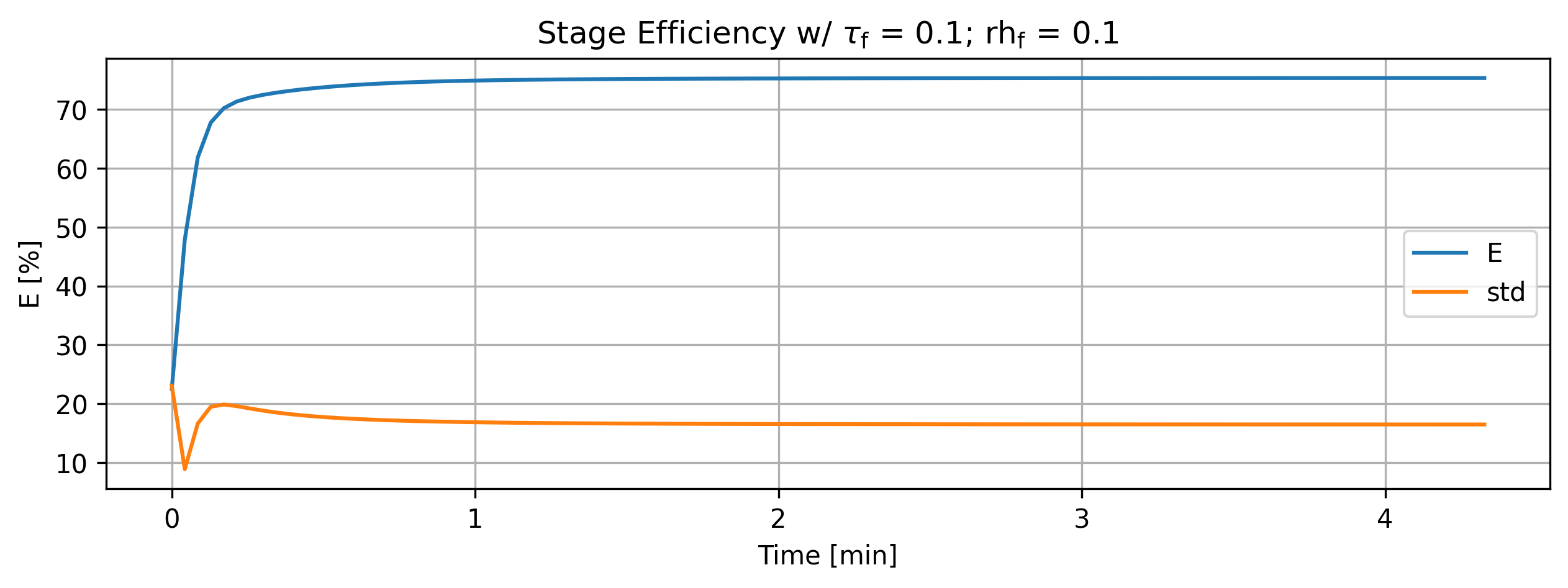
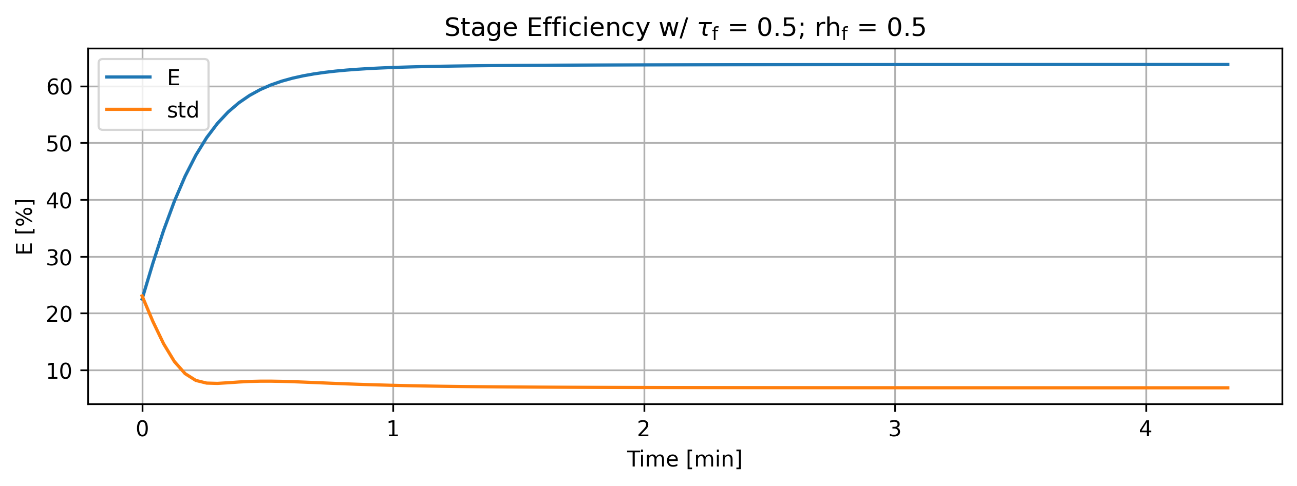
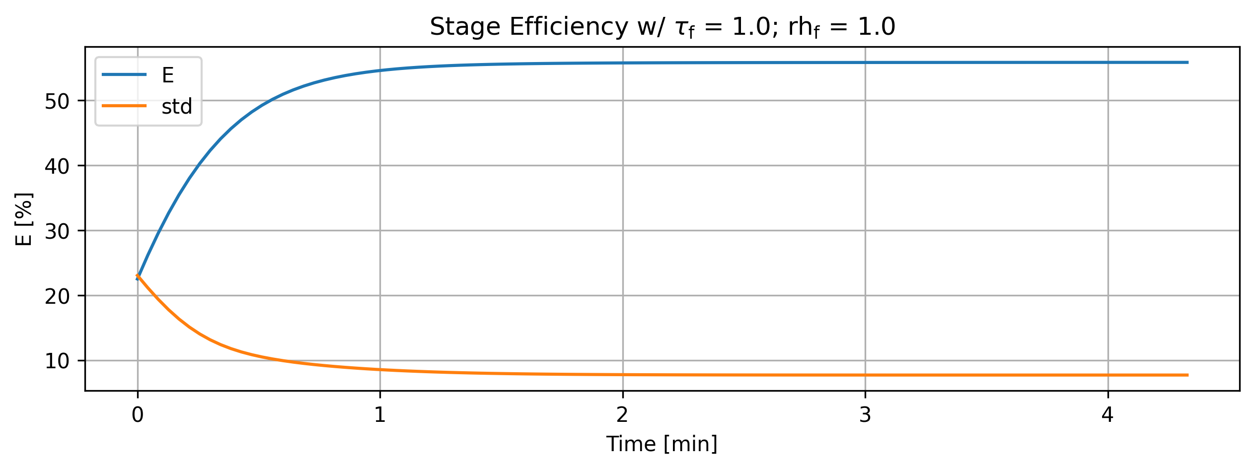
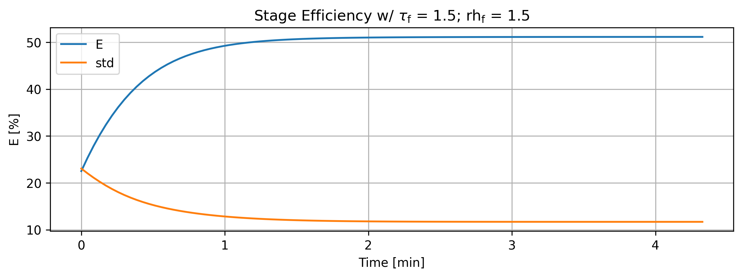
Figure 2: Stage efficiency and deviation variation with parameters.

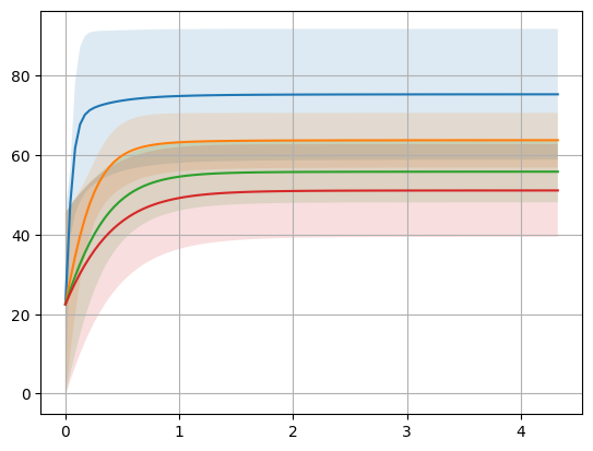
'''For debugging purposes'''
import matplotlib.pyplot as plt
import numpy as np

for eff in efficiencies:
    data = eff.value
    values = list()
    errors = list()
    for entry in data:
        values.append(entry[0])
        errors.append(entry[1])
    values = np.array(values)
    errors = np.array(errors)
    
    plt.plot(data.index/60, values)
    plt.fill_between(data.index/60, values - errors, values + errors, alpha=0.15)
    
plt.grid()

fig_count += 1
print(f'Figure {fig_count}: Multiplot efficiency variation with parameters.')

Figure 3: Multiplot efficiency variation with parameters.

1.3. Inflow Relative Humidity Variation

'''Vary parameter of study'''
stages = list()

inflow_relative_humidity = 25
param_inflow_rh_factors = [0.1, 0.5, 1.0, 1.5] # parameter variation
#param_inflow_rh_factors = [0.2, 1, 1.7, 3.9]


assert len(param_tau_factors) == len(param_inflow_rh_factors)
for param_tau_factor, param_inflow_rh_factor in zip(param_tau_factors, param_inflow_rh_factors):
    
    params['inflow-relative-humidity'] = param_inflow_rh_factor * inflow_relative_humidity
    print('inflow-relative-humidity ', params['inflow-relative-humidity'])
    
    stg = run(params)
    
    stages.append(stg)

if cortix_ai:
    cortix_ai.explain(markdown_display=markdown_display, save_supporting_info=db_save)

inflow-relative-humidity  2.5
Total mass rate density (mixture volume) residual [g/L-s]= -8.99075e-17
total mass inflow rate [g/min]   = 7.471e+02
total mass outflow rate [g/min]  =  7.471e+02
	 net total mass flow rate [g/min] = -3.650e-02
inflow-relative-humidity  12.5
Total mass rate density (mixture volume) residual [g/L-s]= -4.50012e-17
total mass inflow rate [g/min]   = 7.471e+02
total mass outflow rate [g/min]  =  7.471e+02
	 net total mass flow rate [g/min] = -3.650e-02
inflow-relative-humidity  25.0
Total mass rate density (mixture volume) residual [g/L-s]= -2.05998e-17
total mass inflow rate [g/min]   = 7.471e+02
total mass outflow rate [g/min]  =  7.471e+02
	 net total mass flow rate [g/min] = -3.650e-02
inflow-relative-humidity  37.5
Total mass rate density (mixture volume) residual [g/L-s]= -3.07371e-17
total mass inflow rate [g/min]   = 7.471e+02
total mass outflow rate [g/min]  =  7.471e+02
	 net total mass flow rate [g/min] = -3.649e-02
Cortix AI assistant: working on explanation...

Overview

This snippet performs a parameter sweep over a list of multiplicative factors for an “inflow-relative-humidity” parameter, runs a simulation/processing routine for each parameter set, and collects the results.

Variables and initial setup

• A new list stages is created to collect outputs.

• inflow_relative_humidity is set to the baseline value 25 (an integer).

• param_inflow_rh_factors is a list of multiplicative factors [0.1, 0.5, 1.0, 1.5] used to scale the baseline humidity.

• An assertion checks that param_tau_factors and param_inflow_rh_factors have equal length; param_tau_factors is expected to be defined elsewhere (it is not shown in the snippet).

• The snippet relies on several external names that must exist in the surrounding scope: params (a dict-like object), run (a callable), cortix_ai, markdown_display, and db_save.

Main loop behavior

• The loop iterates over pairs produced by zip(param_tau_factors, param_inflow_rh_factors). For each iteration:

  • param_tau_factor and param_inflow_rh_factor are bound to the corresponding elements from the two lists.

  • params[‘inflow-relative-humidity’] is set to param_inflow_rh_factor * inflow_relative_humidity (a numeric multiplication producing a float).

  • The new value of params[‘inflow-relative-humidity’] is printed.

  • run(params) is called and its return value is stored in stg.

  • stg is appended to the stages list.

• Note: param_tau_factor is iterated but not referenced inside the loop body; it is present in the zip to keep iteration counts aligned with param_tau_factors.

After the loop

• If cortix_ai evaluates as truthy, cortix_ai.explain(markdown_display=markdown_display, save_supporting_info=db_save) is invoked. (No explanation of what that call does is provided here.)

• The stages list contains one element per iteration (each element is the stg returned by run(params)).

Side effects, types, and assumptions

• Side effects:

  • params is mutated in-place on each iteration (its ‘inflow-relative-humidity’ key is overwritten).

  • The code prints the currently set inflow-relative-humidity each iteration.

  • run(params) is invoked repeatedly and may have its own side effects.

• Types and values:

  • param_inflow_rh_factors contains floats; multiplying by an integer baseline yields floats.

  • stages becomes a list of whatever objects run(params) returns.

• Preconditions and potential runtime errors:

  • param_tau_factors must be defined and have the same length as param_inflow_rh_factors, otherwise the assert will raise or NameError will occur.

  • params, run, cortix_ai, markdown_display, and db_save must be defined in the surrounding context for the snippet to run without NameError.

AI Parameters:
+ LLM model (OpenAI) = gpt-5-mini
+ LLM cleverness     = 1.0
+ Total # of tokens  = 3312

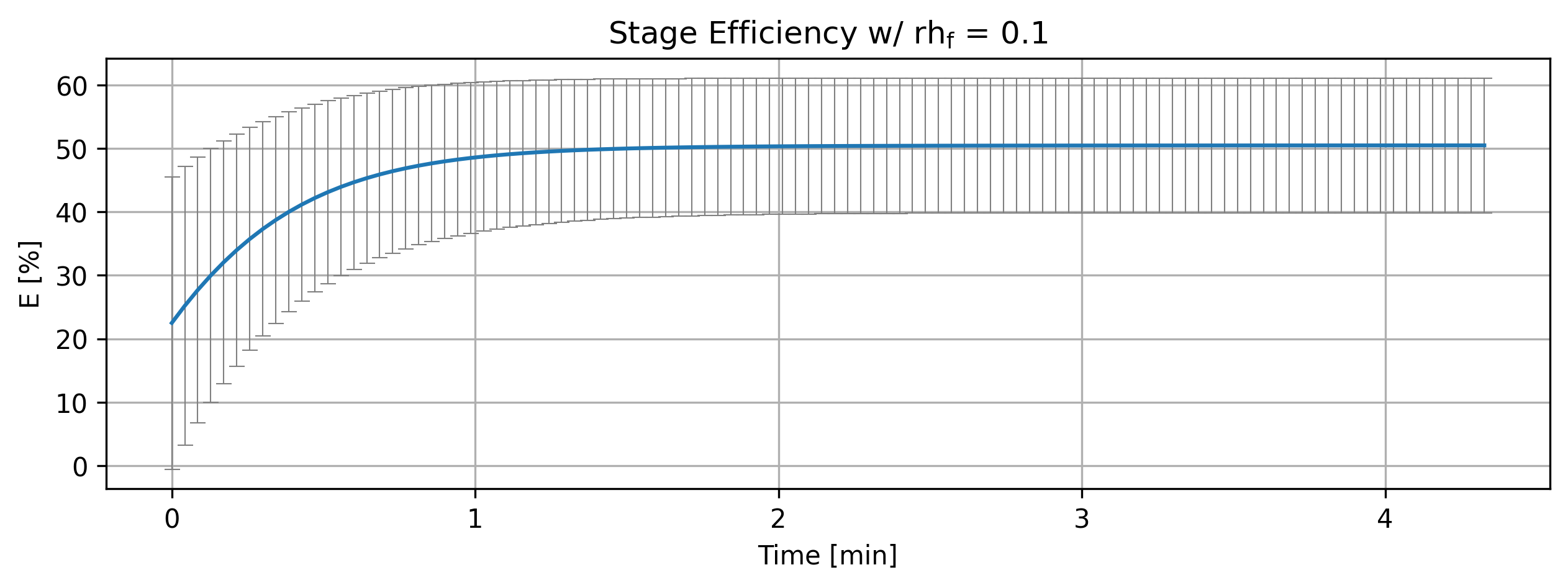
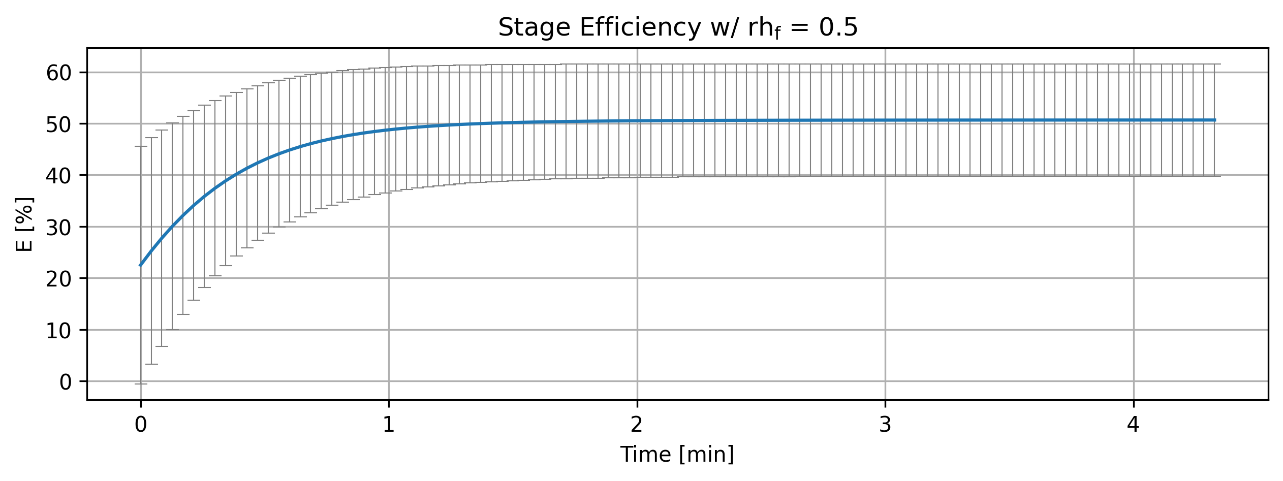
1.3.1. Overall Stage Efficiency

Parameter variation impact on stage efficiency.

'''Stage overall efficiency'''
from cortix import Units as unit
import matplotlib.pyplot as plt

efficiencies = list()

for stg in stages:
    efficiencies.append(stg.efficiency_history(mean=True))

for eff, rh in zip(efficiencies, param_inflow_rh_factors):
    quant = eff
    # Edit quant for AI use below
    quant.name += f"""; @ parameter tau factor = {tau} and parameter relative humidity {rh}"""
    quant.value.name = quant.name
    quant.plot(title=r'Stage Efficiency w/ rh$_{\mathrm{f}}$ = %2.1f'%(rh), x_scaling=1/unit.min, x_label='Time [min]', y_label=quant.latex_name+
               ' ['+quant.unit+']', show=True, figsize=[10,3], error_data=True, error_fill=False)
if cortix_ai: 
    cortix_ai.explain(markdown_display=markdown_display, save_supporting_info=db_save)

fig_count += 1
print(f'Figure {fig_count}: Stage efficiency variation with parameters.')

Cortix AI assistant: working on explanation...

Overview

This snippet collects stage efficiency histories, annotates each history with parameter metadata, plots each history (scaled to minutes), optionally invokes a cortix_ai helper, increments a figure counter, and prints a caption-like summary.

Step-by-step behavior

• The code imports Units from cortix as unit and matplotlib.pyplot as plt.

• It creates an empty list efficiencies.

• It iterates over an iterable stages and appends stg.efficiency_history(mean=True) for each stage to efficiencies.

• It loops over the paired sequences efficiencies and param_inflow_rh_factors using zip, giving eff and rh for each iteration.

  • It assigns eff to local name quant (alias).

  • It mutates quant.name by appending a formatted metadata suffix that embeds the current tau and rh values.

  • It sets quant.value.name equal to the new quant.name (propagating the label into the value object).

  • It calls quant.plot(…) with:

    • title built using a raw string and old-style % formatting to insert rh into the title text (includes LaTeX-like fragment rh$_{\mathrm{f}}$).

    • x_scaling=1/unit.min to convert the x-axis units to minutes.

    • x_label set to ‘Time [min]’.

    • y_label constructed from quant.latex_name and quant.unit.

    • show=True so the plot is displayed when plot executes.

    • figsize=[10,3] for the plot figure size.

    • error_data=True and error_fill=False to control error representation.

• If cortix_ai is truthy, the code calls cortix_ai.explain(markdown_display=markdown_display, save_supporting_info=db_save).

• It increments fig_count by 1 and prints a short line with the updated figure number and a brief description.

Key objects and attributes referenced

• stages: iterable of stage-like objects; each stage provides an efficiency_history(mean=True) method.

• stg.efficiency_history(mean=True): returns an object (here aliased quant) that is expected to have at least these attributes/methods:

  • name: a string label that the code mutates.

  • value: an object with a name attribute (the code sets quant.value.name).

  • latex_name: string used for y-axis label content.

  • unit: string used for y-axis unit display.

  • plot(…): a plotting method that accepts title, x_scaling, x_label, y_label, show, figsize, error_data, and error_fill among others.

• param_inflow_rh_factors: iterable providing rh values zipped with efficiencies.

• tau: external variable whose value is interpolated into quant.name (assumed defined elsewhere in the surrounding scope).

• unit.min: a unit object representing minutes; used by x_scaling=1/unit.min to rescale the plot x axis to minutes.

• cortix_ai, markdown_display, db_save: names in the outer scope; cortix_ai is tested for truthiness and then cortix_ai.explain(…) is invoked (behavior of explain() is not described here).

• fig_count: integer in the outer scope incremented by this snippet and used in the printed summary.

Side effects produced by this snippet

• Mutates quant.name and quant.value.name for each plotted efficiency history.

• Produces one plot per paired (efficiency, rh) item via quant.plot(…) with immediate display (show=True).

• Optionally invokes cortix_ai.explain(…) when cortix_ai is truthy.

• Increments the external fig_count variable and prints a summary line indicating the new figure number.

AI Parameters:
+ LLM model (OpenAI) = gpt-5-mini
+ LLM cleverness     = 1.0
+ Total # of tokens  = 3585
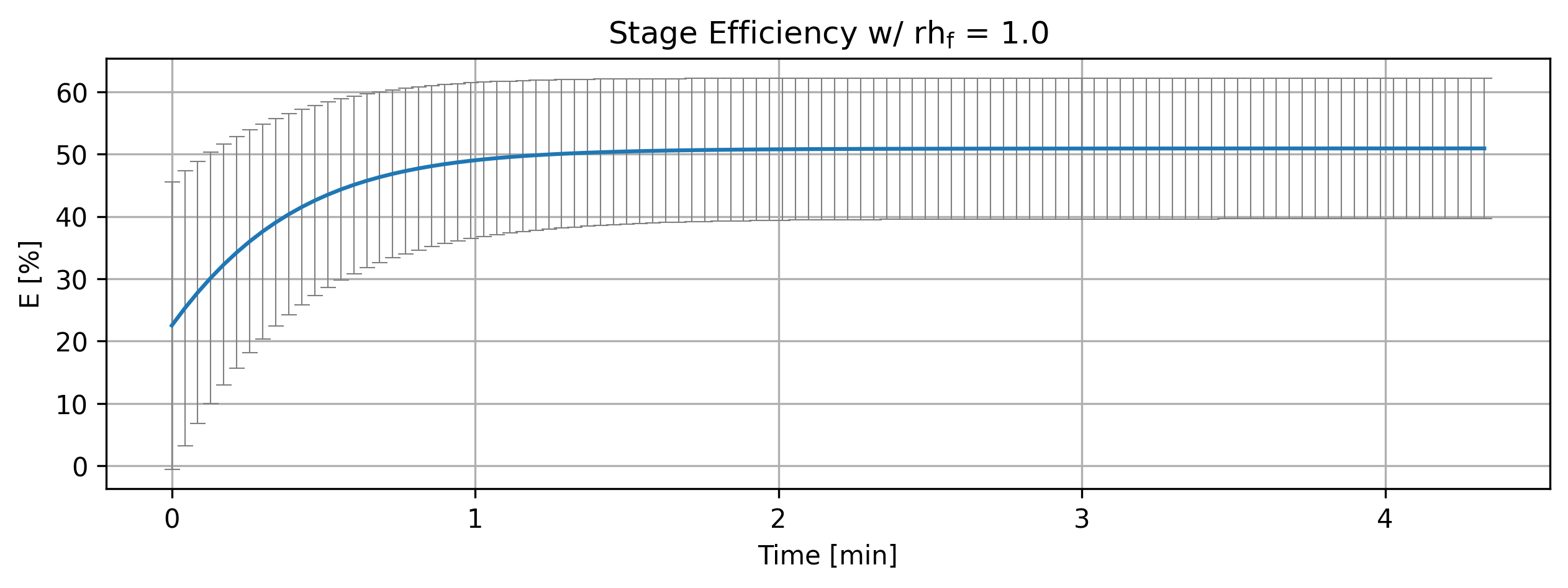
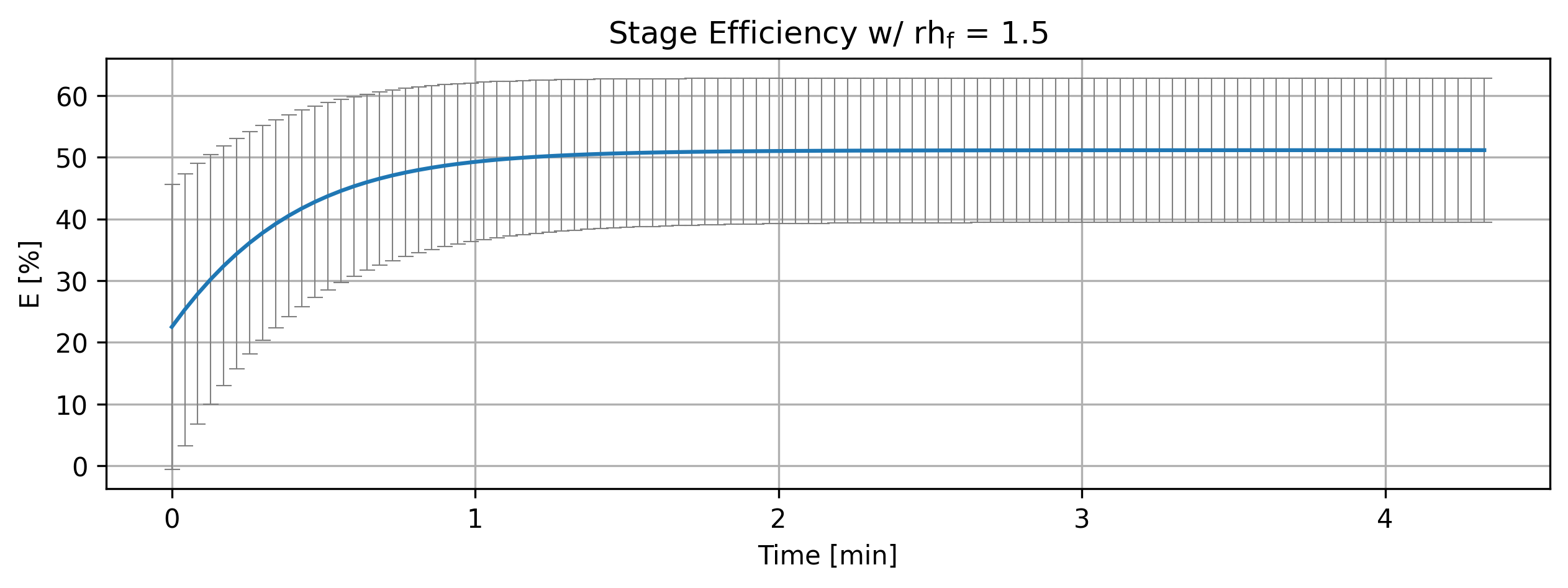
Figure 4: Stage efficiency variation with parameters.

1.3.2. Analysis

LLM analysis.

'''Analyze efficiencies'''
if cortix_ai: 
    cortix_ai.explain(quant=efficiencies, markdown_header_level='<h4>', markdown_display=markdown_display, save_supporting_info=db_save)

Cortix AI assistant: working on explanation...

Overview

• Four time-series show Stage Efficiency (mean and standard deviation [%]) at tau factor = 1.5 for relative humidity (RH) = 0.1, 0.5, 1.0, 1.5.

• Each table columns: index (row id), time [s] (uniform steps of 15.4228 s), column “0” = mean efficiency [%], column “1” = standard deviation [%].

• Common qualitative pattern: mean efficiency rises from an initial ~22.5% toward a plateau ≈50–51% while the standard deviation falls from ≈23% to ≈10–12%.

Time / index column analysis

• Time values are evenly spaced: 0, 15.4228, 30.8457, …, 246.765 s (increment = 15.4228 s).

• Index column is a simple row identifier (0..16) and maps directly to the time steps.

Mean-efficiency (column 0) behavior

• Common transient: rapid increase during the first ≈4–7 steps, then asymptotic approach to a steady value.

• Numerical endpoints (mean at t = 0 and t = 246.765 s):

  • RH = 0.1: 22.5 -> 50.4771 (Δ ≈ +27.98)

  • RH = 0.5: 22.5 -> 50.6654 (Δ ≈ +28.17)

  • RH = 1.0: 22.5 -> 50.9007 (Δ ≈ +28.40)

  • RH = 1.5: 22.5 -> 51.1360 (Δ ≈ +28.64)

• Effect of RH on means:

  • Higher RH yields slightly larger mean at all nonzero times. Example at t = 15.4228 s: means = [35.7254, 35.8446, 35.9937, 36.1428] for RH = [0.1,0.5,1.0,1.5].

  • Long-time plateau increases modestly with RH (~0.66 percentage-point difference between RH 0.1 and 1.5).

• Time-to-plateau:

  • Means reach ≈50% by roughly t ≈ 92.5 s (index 6) for all RH, with higher RH slightly exceeding 50 earlier and by a larger margin.

Standard-deviation (column 1) behavior

• Common transient: std drops steadily from an initial ≈23.0489% toward a lower steady value.

• Numerical endpoints (std at t = 0 and t = 246.765 s):

  • RH = 0.1: 23.0489 -> 10.6134 (Δ ≈ −12.4355)

  • RH = 0.5: 23.0489 -> 10.9095 (Δ ≈ −12.1394)

  • RH = 1.0: 23.0489 -> 11.2907 (Δ ≈ −11.7582)

  • RH = 1.5: 23.0489 -> 11.6832 (Δ ≈ −11.3657)

• Effect of RH on uncertainty:

  • Higher RH corresponds to a consistently larger standard deviation at each time step (e.g., at t = 15.4228 s std = [17.5673, 17.6917, 17.8508, 18.0137] for increasing RH).

  • Long-time std rises with RH from ≈10.61% (RH 0.1) to ≈11.68% (RH 1.5) — a modest increase (~1.07 percentage points).

Comparative summary and interpretation

• All four series share the same initial state and identical time sampling; differences arise only from relative humidity.

• Mean efficiency:

  • Increases strongly from the initial value and then plateaus near 50–51%.

  • Higher RH yields a slightly higher plateau and slightly faster approach to that plateau.

• Variability (std):

  • Decreases substantially from the initial high uncertainty and stabilizes at a lower value.

  • Higher RH leaves a higher residual uncertainty at long times.

• Magnitude of RH effect:

  • Plateau mean shifts by ≲0.7 percentage points across the RH range (0.1 -> 1.5).

  • Long-time standard deviation shifts by ≈1.07 percentage points across the same RH range.

• Practical takeaway:

  • RH produces small but systematic changes: higher RH raises both the steady-state mean efficiency and the steady-state uncertainty, while the transient dynamics (rise of mean, fall of std) are qualitatively the same for all RH values.

Key numeric highlights

• Time increment: 15.4228 s (constant).

• Mean rise (t = 0 -> final): +~28 percentage points for all RH (small RH dependence).

• Std fall (t = 0 -> final): −~11.4 to −12.4 percentage points (larger absolute drop at lower RH).

• Final values (mean, std) by RH:

  • RH 0.1: (50.48%, 10.61%)

  • RH 0.5: (50.67%, 10.91%)

  • RH 1.0: (50.90%, 11.29%)

  • RH 1.5: (51.14%, 11.68%)

AI Parameters:
+ LLM model (OpenAI) = gpt-5-mini
+ LLM cleverness     = 1.0
+ Total # of tokens  = 6062

'''Stage overall efficiency'''
from cortix import Units as unit
import matplotlib.pyplot as plt

for eff, tau, rh in zip(efficiencies, param_tau_factors, param_inflow_rh_factors):
    quant = eff
    quant.plot(title=r'Stage Efficiency w/ rh$_{\mathrm{f}}$ = %2.1f'%(rh), x_scaling=1/unit.min, x_label='Time [min]', y_label=quant.latex_name+
               ' ['+quant.unit+']', legend=['E', 'std'], show=True, figsize=[10,3], error_data=False, error_fill=False)
fig_count += 1
print(f'Figure {fig_count}: Stage efficiency and deviation variation with parameters.')

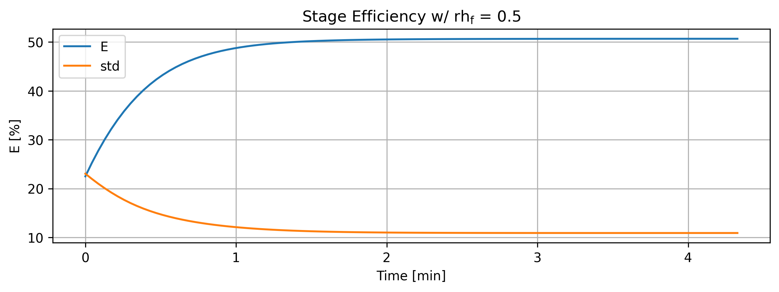
Figure 5: Stage efficiency and deviation variation with parameters.

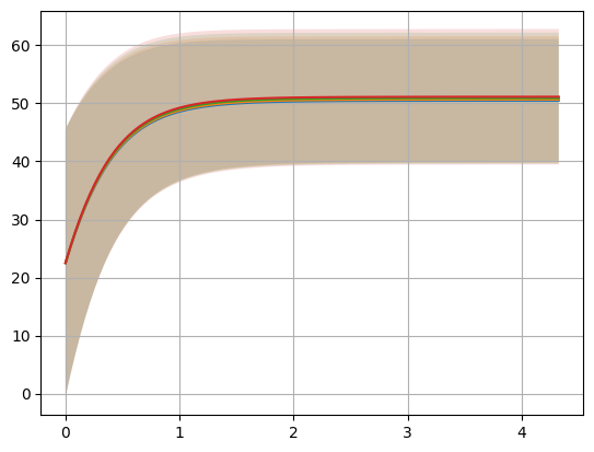
'''For debugging purposes'''
import matplotlib.pyplot as plt
import numpy as np

for eff in efficiencies:
    data = eff.value
    values = list()
    errors = list()
    for entry in data:
        values.append(entry[0])
        errors.append(entry[1])
    values = np.array(values)
    errors = np.array(errors)
    
    plt.plot(data.index/60, values)
    plt.fill_between(data.index/60, values - errors, values + errors, alpha=0.15)
    
plt.grid()

fig_count += 1
print(f'Figure {fig_count}: Multiplot efficiency variation with parameters.')

Figure 6: Multiplot efficiency variation with parameters.